Computation of the gradient for SNE
Many methods exist to visualize high-dimensional data through a two-dimensional map. Those include linear techniques such as PCA and MDS; as well as nonlinear ones such as Isomap, LLE, SNE and t-SNE (resp. Principal Component Analysis, 1933; MultiDimensional Scaling, 1952; Isomap, 2000; Locally Linear Embedding, 2000; Stochastic Neighbor Embedding, 2002; t-Distributed Stochastic Neighbor Embedding, 2008). Some of those dimensionality reduction methods are illustrated in this sklearn example.
A popular method for nonlinear mapping is t-SNE. This method has been developed by Laurens van der Maaten and Geoffrey Hinton in [1]. It is based on SNE and improves it by addressing the “crowding problem” (tendency of mapped points to aggregate into a unique central cluster). You can familiarize yourself with t-SNE here, which allows exploration of various examples interactively.
In this post, we propose to derive gradient of the SNE algorithm (not to be confused with t-SNE, for which gradient calculation is detailed in Appendix A of [1]). SNE gradient is given in both original and t-SNE article, but neither detailed (see Equation 5 of [2], and Section 2 of [1]).
In the following, we describe how works SNE (which is essentially a rewriting of Section 2 of [1]) before deriving SNE gradient step by step.
How works SNE
High-dimensional points
We have points \((x_i)_i\) is an high-dimensional space. We can measure distance between two points \(i\) and \(j\) with \(\| x_i - x_j \|\).
We define the similarity between points \(i\) and \(j\) as a conditional probability:
\[p_{j \mid i} := \frac{\exp \left( - \| x_i - x_j \|^2 / 2 \sigma_i^2 \right)}{\sum_{k \neq i} \exp \left( - \| x_i - x_k \|^2 / 2 \sigma_i^2 \right)}.\]\(p_{j \mid i}\) represents the probability “that \(x_i\) would pick \(x_j\) as its neighbor, if neighbors were picked in proportion to their probability density under a Gaussian centered at \(x_i\)”. We let \(p_{i \mid i}:=0\).
The method for determining \(\sigma_i\) is presented in [1] and is related with the perplexity parameter.
Low-dimensional mapping
We wish to obtain \((y_i)_i\) belonging to a two-dimensional space, where each \(y_i\) represents a point in the plane corresponding to \(x_i\).
We define the similarity between points \(i\) and \(j\) in this space:
\[q_{j \mid i} := \frac{\exp \left( - \| y_i - y_j \|^2 \right)}{\sum_{k \neq i} \exp \left( - \| y_i - y_k \|^2 \right)}.\]We let \(q_{i \mid i}:=0\).
What is a good map from \((x_i)_i\) to \((y_i)_i\)?
A good map from \((x_i)_i\) to \((y_i)_i\) is a map for which distributions \(P_i: j \mapsto p_{j \mid i}\) and \(Q_i: j \mapsto q_{j \mid i}\) are equal (for all \(i\)).
We measure the distance between distributions \(P_i\) and \(Q_i\) with the Kullback-Leibler divergence:
\[\text{KL}(P_i \mid \mid Q_i) = \sum_{j} p_{j \mid i} \log \frac{p_{j \mid i}}{q_{j \mid i}}.\][See this post for more details].
Since we want to minimize them for all \(i\), we finally define the cost function as:
\[C = \sum_i \text{KL}(P_i \mid \mid Q_i).\]Asymmetry of \(\text{KL}\)
We remember that \(\text{KL}\) divergence is asymmetric (see Fig 3.6. from Deep learning book p.74). In SNE, we focus on choosing a distribution \(Q_i\) which fairly represents the whole distribution \(P_i\), so we optimize \(\text{KL}(P_i \mid \mid Q_i)\).
This means:
- If we use widely separated 2D points to represent nearby datapoints, there will be a large cost (i.e. we have a small \(q_{j \mid i}\) to model a large \(p_{j \mid i}\), i.e. the points are far away in \(Y\) but close in \(X\)),
- If we use nearby 2D points to represent widely separated datapoints, there will be a small cost (i.e. we have a large \(q_{j \mid i}\) to model a small \(p_{j \mid i}\), i.e. the points are close in \(Y\) but far away in \(X\)).
On the whole, “the SNE cost function focuses on retaining the local structure of the data in the map”.
Gradient descent
The cost function is optimized with a variant of the classic gradient descent (see [1] for details).
Derivation of the SNE gradient
We have using previous notations:
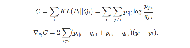
\[C = \sum_{i} KL(P_i || Q_i) = \sum_{i} \sum_{j \neq i} p_{j|i} \log \frac{p_{j|i}}{q_{j|i}}.\]Taking the gradient, we want to compute:
\[-\nabla_{y_l} C = \sum_{i} \sum_{j \neq i} p_{j|i} \frac{\nabla_{y_l} q_{j|i}}{q_{j|i}}.\]Decomposition into 3 terms
We separate the calculation as a sum of 3 terms:
\[-\nabla_{y_l} C = [\text{I}] + [\text{II}] + [\text{III}],\]where \([\text{I}]\) is when \(i=l\); \([\text{II}]\) is when \(j=l\); and \([\text{III}]\) is the remainder term:
\[[\text{I}] := \sum_{j \neq l} p_{j|l} \frac{\nabla_{y_l} q_{j|l}}{q_{j|l}},\] \[[\text{II}] := \sum_{i \neq l} p_{l|i} \frac{\nabla_{y_l} q_{l|i}}{q_{l|i}},\] \[[\text{III}] := \sum_{i \neq l} \sum_{j \neq i,l} p_{j|i} \frac{\nabla_{y_l} q_{j|i}}{q_{j|i}}.\]Calculation of \(q_{j \mid i}\) and \(\nabla_{y_l} q_{j \mid i}\)
We define for all \(k, l\):
\[f_k(y_l) := \exp \left( -||y_l - y_k||^2 \right).\]We have, using \(\nabla_{a} \| a - b \|^2 = 2(a-b)\):
\[\nabla_{y_l} f_k(y_l) = -2(y_l - y_k) \exp \left( -||y_l - y_k||^2 \right) = -2(y_l - y_k) f_k(y_l).\]Case \([\text{I}]\):
We have
\[\begin{align} q_{j|l} = \frac{f_j(y_l)}{\sum_{k \neq l} f_k(y_l)} \end{align}\]and
\[\begin{align} \nabla_{y_l} q_{j|l} =& \frac{\nabla_{y_l} f_j(y_l) \sum_{k \neq l} f_k(y_l) - f_j(y_l) \sum_{k \neq l}\nabla_{y_l} f_k(y_l)}{\left( \sum_{k \neq l} f_k(y_l) \right)^2} \\ =& \frac{\nabla_{y_l} f_j(y_l)}{\sum_{k \neq l} f_k(y_l)} - \frac{f_j(y_l) \sum_{k \neq l} \nabla_{y_l} f_k(y_l)}{\left( \sum_{k \neq l} f_k(y_l) \right)^2}. \end{align}\]Case \([\text{II}]\):
We have
\[q_{l|i} = \frac{f_i(y_l)}{f_i(y_l) + \sum_{k \neq \lbrace i, l \rbrace} \exp \left( - ||y_i - y_k ||^2 \right)} =: \frac{f_i(y_l)}{f_i(y_l) + B}\]and
\[\begin{align} \nabla_{y_l} q_{l|i} =& \frac{(f_i(y_l) + B) \nabla_{y_l} f_i(y_l) - f_i(y_l) \nabla_{y_l} f_i(y_l)}{ \left( \sum_{k \neq i} \exp \left( - ||y_i - y_k||^2 \right) \right)^2} \\ =:& \frac{S \nabla_{y_l} f_i(y_l) - f_i(y_l) \nabla_{y_l} f_i(y_l)}{S^2}. \end{align}\]Case \([\text{III}]\):
We have
\[q_{j|i} = \frac{\exp(-||y_i - y_j||^2)}{f_i(y_l) + \sum_{k \neq \lbrace i, l \rbrace} \exp \left( -||y_i - y_k||^2 \right)} =: \frac{A}{f_i(y_l) + B}\]and
\[\begin{align} \nabla_{y_l} q_{j|i} = \frac{-A \nabla_{y_l} f_i(y_l)}{\left( f_i(y_l) + B \right)^2} = \frac{2 A (y_l - y_i) f_i(y_l)}{S^2}. \end{align}\]Calculation of \([\text{I}]\)
\[\begin{align} [\text{I}] =& \sum_{j \neq l} p_{j|l} \frac{\nabla_{y_l} q_{j|l}}{q_{j|l}} \\ =& \sum_{j \neq l} p_{j|l} \frac{\sum_{k \neq l} f_k(y_l)}{f_j(y_l)} \left( \frac{\nabla_{y_l} f_j(y_l)}{\sum_{k \neq l} f_k(y_l)} - \frac{f_j(y_l) \sum_{k \neq l} \nabla_{y_l} f_k(y_l)}{\left( \sum_{k \neq l} f_k(y_l) \right)^2} \right) \\ =& \sum_{j \neq l} p_{j|l} \left( \frac{\nabla_{y_l} f_j(y_l)}{f_j(y_l)} - \frac{\sum_{k \neq l} \nabla_{y_l} f_k(y_l)}{\sum_{k \neq l} f_k(y_l) } \right) \\ =& \sum_{j \neq l} p_{j|l} \left( -2(y_l - y_j) + \frac{\sum_{k \neq l} 2(y_l - y_k) f_k(y_l)}{\sum_{k \neq l} f_k(y_l) } \right) \\ =& - 2 \sum_{j \neq l} p_{j|l} (y_l - y_j) + 2 \sum_{j \neq l} p_{j|l} \left( \sum_{k \neq l} (y_l - y_k) \frac{f_k(y_l)}{\sum_{k \neq l} f_k(y_l)} \right). \end{align}\]But \(q_{k \mid l} = \frac{f_k(y_l)}{\sum_{k \neq l} f_k(y_l)}\) so:
\[[\text{I}] = - 2 \sum_{j \neq l} p_{j|l} (y_l - y_j) + 2 \left( \sum_{k \neq l} (y_l - y_k) q_{k|l} \right) \left( \sum_{j \neq l} p_{j|l} \right),\]and \(\sum_{j \neq l} p_{j \mid l} = 1\), then:
\[\begin{align} [\text{I}] =& - 2 \sum_{j \neq l} p_{j|l} (y_l - y_j) + 2 \sum_{k \neq l} (y_l - y_k) q_{k|l} \\ =& - 2 \sum_{i \neq l} p_{i|l} (y_l - y_i) + 2 \sum_{i \neq l} (y_l - y_i) q_{i|l}. \end{align}\]Calculation of \([\text{II}]\)
\[\begin{align} [\text{II}] =& \sum_{i \neq l} p_{l|i} \frac{\nabla_{y_l} q_{l|i}}{q_{l|i}} \\ =& \sum_{i \neq l} p_{l|i} \left( \frac{f_i(y_l) + B}{f_i(y_l)} \right) \left( \frac{S \nabla_{y_l} f_i(y_l) - f_i(y_l) \nabla_{y_l} f_i(y_l)}{S^2} \right). \end{align}\]Since \(S = f_i(y_l) + B\), we have:
\[\begin{align} [\text{II}] =& \sum_{i \neq l} p_{l|i} \left( \frac{\nabla_{y_l} f_i(y_l)}{f_i(y_l)} - \frac{\nabla_{y_l} f_i(y_l)}{S} \right) \\ =& \sum_{i \neq l} p_{l|i} \left( - 2(y_l - y_i) + 2 (y_l - y_i) \frac{f_i(y_l)}{S} \right). \end{align}\]But \(q_{l \mid i} = \frac{f_i(y_l)}{S}\), so:
\[[\text{II}] = -2 \sum_{i \neq l} p_{l|i} (y_l - y_i) + 2 \sum_{i \neq l} p_{l|i} (y_l - y_i) q_{l|i}.\]Calculation of \([\text{III}]\)
\[\begin{align} [\text{III}] =& \sum_{i \neq l} \sum_{j \neq i,l} p_{j|i} \frac{\nabla_{y_l} q_{j|i}}{q_{j|i}} \\ =& \sum_{i \neq l} \sum_{j \neq i,l} p_{j|i} \left( \frac{f_i(y_l) + B}{A} \right) \left( \frac{2A (y_l - y_i) f_i(y_l)}{S^2} \right). \end{align}\]Since \(S = f_i(y_l) + B\), we have:
\[[\text{III}] = 2 \sum_{i \neq l} \sum_{j \neq i,l} p_{j|i} \left( \frac{(y_l - y_i) f_i(y_l)}{S} \right).\]But \(q_{l \mid i} = \frac{f_i(y_l)}{S}\), so:
\[\begin{align} [\text{III}] =& 2 \sum_{i \neq l} \sum_{j \neq i,l} p_{j|i} (y_l - y_i) q_{l|i} \\ =& 2 \sum_{i \neq l} \left[ (y_l - y_i) q_{l|i} \left( \sum_{j \neq i,l} p_{j|i} \right) \right]. \end{align}\]We have: \(\sum_{j \neq i, l} p_{j \mid i} = 1 - p_{l \mid i}\), so finally:
\[[\text{III}] = 2 \sum_{i \neq l} (y_l - y_i) q_{l|i} \left( 1 - p_{l|i} \right).\]Final form of the gradient
\[\begin{align} -\nabla_{y_l} C = & [\text{I}] + [\text{II}] + [\text{III}] \\ = &- 2 \sum_{i \neq l} p_{i|l} (y_l - y_i) + 2 \sum_{i \neq l} (y_l - y_i) q_{i|l} -2 \sum_{i \neq l} p_{l|i} (y_l - y_i) \\ &+ 2 \sum_{i \neq l} p_{l|i} (y_l - y_i) q_{l|i} + 2 \sum_{i \neq l} (y_l - y_i) q_{l|i} \left( 1 - p_{l|i} \right) \end{align}\]So after simplification:
\[\begin{align} -\nabla_{y_l} C = &- 2 \sum_{i \neq l} p_{i|l} (y_l - y_i) + 2 \sum_{i \neq l} (y_l - y_i) q_{i|l} \\ &- 2 \sum_{i \neq l} p_{l|i} (y_l - y_i) + 2 \sum_{i \neq l} (y_l - y_i) q_{l|i} \end{align}\]and finally:
\[\nabla_{y_l} C = 2 \sum_{i \neq l} (p_{i|l} - q_{i|l} + p_{l|i} - q_{l|i})(y_l - y_i).\]The form of this gradient is interpreted in Section 2 of [1].