An illustration of Metropolis–Hastings algorithm
Metropolis–Hastings algorithm is a method for sampling from a probability distribution. It is used when direct sampling is difficult.
This post illustrates the algorithm by sampling from \(\mathcal{N}(. \mid > 5)\) – the univariate normal distribution conditional on being greater than \(5\). This example has been chosen for its simplicity, for understanding how the algorithm actually works.
For real applications, other methods are preferred for sampling \(\mathcal{N}(. \mid > l)\): It is direct for \(l = 5\), and more tricky when \(l\) is larger than \(10\). You can read this Wikipedia section for details.
Simulation code has been written in R and is available at that address.
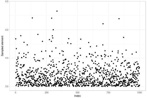
Fig. 1. Sample of size 1000 of a truncated normal distribution drawn with Metropolis–Hastings algorithm
Presentation
The aim of the algorithm is to simulate a sample following a distribution (target distribution). We assume that this target distribution has a density, and that we know it up to a multiplicative constant. This means that we do not need to know exactly the normalization constant, which can be difficult to approximate for rare events or high-dimensional densities.
The idea is to perform simulations through another distribution (instrumental distribution). This instrumental distribution is chosen to be easy to sample.
The simulations computed through the instrumental distribution are “corrected”. To this end, we construct a Markov chain which admits a unique stationary distribution which is the target distribution. In practice, steps of the chain follows the instrumental distribution, but step can be rejected with a certain probability.
Illustrative example – Preparation
In this example, we want to simulate a sample of the standard normal distribution knowing that the values are greater than a limit \(5\). If we want to obtain this sample directly by reject algorithm, most of values are rejected:
set.seed(2713)
limit = 5
x_test = rnorm(10000)
max(x_test) # close to 3.5
which(x_test > limit) # no element, all are rejected
Target distribution. Therefore, we will use a Metropolis–Hastings algorithm to sample this distribution. We first need the density of the target distribution up to a constant. This is easily available, by cutting the normal distribution:
# Target density (this density is only known up to a constant)
pi_func0 = function(x, limit) {
  if(x < limit) {
    return(0)
  } else {
    return(dnorm(x, mean = 0, sd = 1))
  }
}
pi_func = function(x) {pi_func0(x, limit)}
Instrumental distribution. Then, we need an instrumental distribution \(q(. \mid x)\) which can be easily simulated. Here, the normal distribution centered in \(x\) and with standard deviation of \(0.01\) is selected. Sampling from this distribution is easy.
# Simulation of the instrumental distribution
q_func_symm = function(x, sd = 0.01) {
  y = rnorm(1, x, sd)
  return(y)
}
Note that this instrumental distribution is symmetric. This is not a requirement for Metropolis–Hastings algorithm, but simplifies computations a lot. In particular, density of the instrumental distribution is not needed in this case (we only need to know how to sample from it). The algorithm is sometimes called Metropolis algorithm in this particular case.
In the previous instrumental distribution,
parameter sd indicates range of each step. When sd is small, each
step is small and the probability to be accepted is large. However, the
Markov chain is moving slowly and many steps are necessary to reach
stationary distribution. When sd is large, larger steps are done, but are
accepted less often.
Markov process
We construct a Markov chain \((x(t))_{t}\). It is designed to have a unique stationary distribution which is the target distribution. You can read Section 2.1 of this course for formal derivation. As a consequence, given \(T\) a large number, \(x(T)\) can be regarded as a sample element from target distribution (and we hope that \(T\) is not so large…).
Let’s construct the Markov chain in our example. Given \(x(t)\) for any \(t \geq 1\), we use the following function to compute \(x(t+1)\). Basicly, we simulate one element \(y\) from \(q(. \mid x(t))\), the instrumental distribution given \(x(t)\); then accept it with a certain probability \(\alpha(x(t),y)\)
iterate_t_to_t_plus_1 = function(x_t, sd) {
  y_t_plus_1 = q_func_symm(x_t, sd)
  alpha_current = alpha(x_t, y_t_plus_1)
  x_t_plus_1 = NA
  if(runif(1) < alpha_current) { # move
    x_t_plus_1 = y_t_plus_1
  } else { # reject
    x_t_plus_1 = x_t
  }
  return(x_t_plus_1)
}
It remains to define the probability \(\alpha(x(t),y)\) to accept the move. It is simply the quotient of probability of the target distribution (it is a little more complex when instrumental distribution is not symmetric).
alpha = function(x_t, y_t_plus_1) {
  alpha_out = min(pi_func(y_t_plus_1) / pi_func(x_t), 1)
  return(alpha_out)
}
Illustrative example – Computations
In this section, we sample \(\mathcal{N}(. \mid > 5)\) using Metropolis–Hastings algorithm. We define length of the chain, the parameter of standard deviation in the instrumental distribution, and the initial state.
N = 1000000 # length of the chain
sd = 3 # standard deviation of the steps move
x_1 = limit # initialization of the chain
We compute a chain until step \(N\) for a certain alea \(\omega\).
x_t_vect = rep(NA, N)
x_t_vect[1] = x_1
for(i in 2:N) {
  if(i %% 10000 == 0) {
    print(i)
  }
  x_t_vect[i] = iterate_t_to_t_plus_1(x_t_vect[i-1], sd)
}
Two consecutives elements of the chain are correlated. This issue is inherent in MCMC methods.
We obtain an almost uncorrelated sample by selecting a subset of \(x(t)\).
For example, if we know that the chain has almost reached stationarity after a certain number of steps s, then we can select \(x(s)\), \(x(2s)\), \(x(3s)\).
In our case, the number of steps to wait depends on the sd parameter.
In the following, we took step=1000.
step = 1000
simulated_distr = x_t_vect[seq(from = step,
                               by = step,
                               to = length(x_t_vect))]
The final sample has length \(N/step\) and follows \(\mathcal{N}(. \mid > 5)\) (almost).
The following figure compares sample obtained from Metropolis–Hastings algorithm with sample obtained from direct formula using inverse transform method (see Wikipedia page).
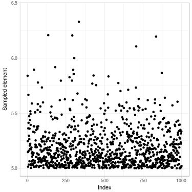
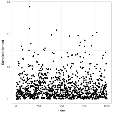
Fig. 2. Sample of size 1000 drawn of a truncated normal distribution. (Left) Using Metropolis–Hastings algorithm (Right) Directly using inverse transform method
Visually, it looks good. Further checking are necessary, especially by checking autocorrelation of the sample.