Periodic mixtures
Let \(f\) be a real function. For \(\lambda > 0\), we are interested in the equally-spaced summation \(\sum_{k=-\infty}^{+\infty} f(.+k\lambda)\), that can be interpreted depending on the context as a periodic mixture or as a wrapped distribution. For some specific functions such as the Gaussian density, we derive expressions, evaluations, and approximations of the sum, further accompanied with visualization of the different shapes for various values of \(\lambda\).
Base functions \(f_{\sigma}\)
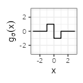
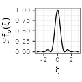
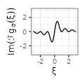
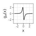
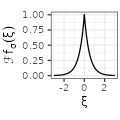
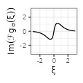
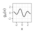
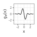
In the following, we consider seven types of functions \(f_{\sigma}\), each type being parametrized by \(\sigma>0\) representing a kind of deviation. The types are named Rectangular, Linear, Exponential, Polynomial, Gaussian, Sinc, and Sincsquare, and correspond to family of densities, except for Sinc that however still sums to one. The definition of the functions is provided in the table below. As we can see, each function is adjusted to peak at \(x=0\) and then symmetrically fade to zero.
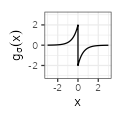
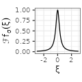
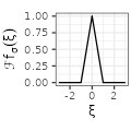
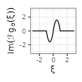
For each type, we complement the table with additional columns derived from the function \(f_{\sigma}\), by considering the derivative of the functions \(g(x) := f'(x)\) and their Fourier transforms. We use below the conventions \(\mathcal{F}f(\xi) := \int_{-\infty}^{+\infty} f(x) e^{-2i\pi x \xi} dx\) and \(\text{sinc}(x) := \frac{\sin(\pi x)}{\pi x}.\)
In the visual representations of the table, the value of \(\sigma\) is set to one, as indicated in the first column, and corresponds to the case where the Fourier transform also sums to one (or equivalently where \(f(0) = 1\)).
| $$\text{type}$$ | $$~~~~~~~~~~f_{\sigma}(x)~~~~~~~~~~$$ | $$~~~~~~~~~~g_{\sigma}(x)~~~~~~~~~~$$ | $$~~~~~~~~~\mathcal{F}f_{\sigma}(\xi)~~~~~~~~~$$ | $$~~~~~~~~~\mathcal{F}g_{\sigma}(\xi)~~~~~~~~~$$ |
| Rectangular$$(\sigma=1)$$ | 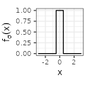 $${\scriptstyle \sigma^{-1} \mathbf{1}_{|x| \leq \sigma/2}}$$ $${\scriptstyle \sigma^{-1} \mathbf{1}_{|x| \leq \sigma/2}}$$ |
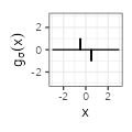 $${\scriptstyle \sigma^{-1} \left( \delta_{x = -\sigma/2} - \delta_{x = \sigma/2} \right) }$$ $${\scriptstyle \sigma^{-1} \left( \delta_{x = -\sigma/2} - \delta_{x = \sigma/2} \right) }$$ |
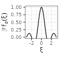 $${\scriptstyle \text{sinc}(\sigma \xi)}$$ $${\scriptstyle \text{sinc}(\sigma \xi)}$$ |
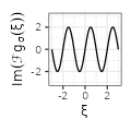 $${\scriptstyle 2\pi i \xi \text{sinc}(\sigma \xi)}$$ $${\scriptstyle 2\pi i \xi \text{sinc}(\sigma \xi)}$$ |
| Linear$$(\sigma=1)$$ | 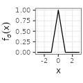 $${\scriptstyle \sigma^{-1} \left( 1- \frac{|x|}{\sigma} \right) \mathbf{1}_{|x| \leq \sigma}}$$ $${\scriptstyle \sigma^{-1} \left( 1- \frac{|x|}{\sigma} \right) \mathbf{1}_{|x| \leq \sigma}}$$ |
 $${\scriptstyle - \frac{\text{sign}(x)}{\sigma^2} \mathbf{1}_{|x| \leq \sigma}}$$ $${\scriptstyle - \frac{\text{sign}(x)}{\sigma^2} \mathbf{1}_{|x| \leq \sigma}}$$ |
 $${\scriptstyle \text{sinc}^2(\sigma \xi)}$$ $${\scriptstyle \text{sinc}^2(\sigma \xi)}$$ |
 $${\scriptstyle 2\pi i \xi \text{sinc}^2(\sigma \xi)}$$ $${\scriptstyle 2\pi i \xi \text{sinc}^2(\sigma \xi)}$$ |
| Exponential$$(\sigma=1)$$ | 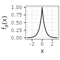 $${\scriptstyle \sigma^{-1} e^{-\frac{2|x|}{\sigma}}}$$ $${\scriptstyle \sigma^{-1} e^{-\frac{2|x|}{\sigma}}}$$ |
 $${\scriptstyle - \frac{2 \text{sign}(x)}{\sigma^2} e^{-\frac{2|x|}{\sigma}}}$$ $${\scriptstyle - \frac{2 \text{sign}(x)}{\sigma^2} e^{-\frac{2|x|}{\sigma}}}$$ |
 $${\scriptstyle \frac{1}{1 + \left( \pi \sigma \xi \right)^2}}$$ $${\scriptstyle \frac{1}{1 + \left( \pi \sigma \xi \right)^2}}$$ |
 $${\scriptstyle 2\pi i \xi \frac{1}{1 + \left( \pi \sigma \xi \right)^2}}$$ $${\scriptstyle 2\pi i \xi \frac{1}{1 + \left( \pi \sigma \xi \right)^2}}$$ |
| Polynomial$$(\sigma=1)$$ |  $${\scriptstyle \sigma^{-1} \frac{1}{1 + \left( \pi x/\sigma \right) ^2}}$$ $${\scriptstyle \sigma^{-1} \frac{1}{1 + \left( \pi x/\sigma \right) ^2}}$$ |
 $${\scriptstyle -2 \pi^2 \sigma^{-3} \frac{x}{\left( 1 + \left( \pi x/\sigma \right)^2 \right)^2} }$$ $${\scriptstyle -2 \pi^2 \sigma^{-3} \frac{x}{\left( 1 + \left( \pi x/\sigma \right)^2 \right)^2} }$$ |
 $${\scriptstyle e^{-2 \sigma |\xi|}}$$ $${\scriptstyle e^{-2 \sigma |\xi|}}$$ |
 $${\scriptstyle 2\pi i \xi e^{-2 \sigma |\xi|}}$$ $${\scriptstyle 2\pi i \xi e^{-2 \sigma |\xi|}}$$ |
| Gaussian$$(\sigma=1)$$ | 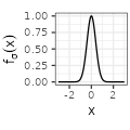 $${\scriptstyle \sigma^{-1} e^{-\frac{\pi x^2}{\sigma^2}}}$$ $${\scriptstyle \sigma^{-1} e^{-\frac{\pi x^2}{\sigma^2}}}$$ |
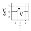 $${\scriptstyle - 2 \pi \sigma^{-3} x e^{-\frac{\pi x^2}{\sigma^2}}}$$ $${\scriptstyle - 2 \pi \sigma^{-3} x e^{-\frac{\pi x^2}{\sigma^2}}}$$ |
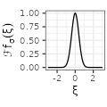 $${\scriptstyle e^{-\pi \sigma^2 \xi^2}}$$ $${\scriptstyle e^{-\pi \sigma^2 \xi^2}}$$ |
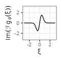 $${\scriptstyle 2\pi i \xi e^{-\pi \sigma^2 \xi^2}}$$ $${\scriptstyle 2\pi i \xi e^{-\pi \sigma^2 \xi^2}}$$ |
| Sinc$$(\sigma=1)$$ | 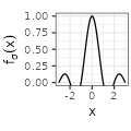 $${\scriptstyle \sigma^{-1} \text{sinc} (x / \sigma)}$$ $${\scriptstyle \sigma^{-1} \text{sinc} (x / \sigma)}$$ |
 $${\scriptstyle \frac{1}{\sigma x} \cos \left( \frac{\pi x}{\sigma} \right) - \frac{1}{\pi x^2} \sin \left( \frac{\pi x}{\sigma} \right)}$$ $${\scriptstyle \frac{1}{\sigma x} \cos \left( \frac{\pi x}{\sigma} \right) - \frac{1}{\pi x^2} \sin \left( \frac{\pi x}{\sigma} \right)}$$ |
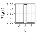 $${\scriptstyle \mathbf{1}_{\xi \in \left[ -\frac{1}{2 \sigma}, \frac{1}{2 \sigma} \right]}}$$ $${\scriptstyle \mathbf{1}_{\xi \in \left[ -\frac{1}{2 \sigma}, \frac{1}{2 \sigma} \right]}}$$ |
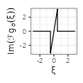 $${\scriptstyle 2 \pi i \xi \mathbf{1}_{\xi \in \left[ -\frac{1}{2 \sigma}, \frac{1}{2 \sigma} \right]}}$$ $${\scriptstyle 2 \pi i \xi \mathbf{1}_{\xi \in \left[ -\frac{1}{2 \sigma}, \frac{1}{2 \sigma} \right]}}$$ |
| Sincsquare$$(\sigma=1)$$ | 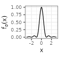 $${\scriptstyle \sigma^{-1} \text{sinc}^2 (x / \sigma)}$$ $${\scriptstyle \sigma^{-1} \text{sinc}^2 (x / \sigma)}$$ |
 $${\scriptstyle \frac{\sin \left( 2 \pi x / \sigma \right)}{\pi x^2} - 2 \sigma \frac{\sin^2 \left( \pi x / \sigma \right)}{\pi^2 x^3}}$$ $${\scriptstyle \frac{\sin \left( 2 \pi x / \sigma \right)}{\pi x^2} - 2 \sigma \frac{\sin^2 \left( \pi x / \sigma \right)}{\pi^2 x^3}}$$ |
 $${\scriptstyle\left( 1- |\xi| \sigma \right) \mathbf{1}_{|\xi| \leq 1/\sigma}}$$ $${\scriptstyle\left( 1- |\xi| \sigma \right) \mathbf{1}_{|\xi| \leq 1/\sigma}}$$ |
 $${\scriptstyle 2 \pi i \xi \left( 1- |\xi| \sigma \right) \mathbf{1}_{|\xi| \leq 1/\sigma}}$$ $${\scriptstyle 2 \pi i \xi \left( 1- |\xi| \sigma \right) \mathbf{1}_{|\xi| \leq 1/\sigma}}$$ |
Sum of the base functions \(S_{\lambda}f_{\sigma}\)
In each case, we are interested in wrapping the function around a circle of circumference \(\lambda > 0\), that is to let, for \(x \in [-\lambda/2,\lambda/2)\), \(S_{\lambda}f(x) := \sum_{k=-\infty}^{+\infty} f(x+k\lambda)\). This function is extended by shifts of \(\lambda\) on the whole real line (which, by periodicity, is also equal to \(S_{\lambda}f(x)\) for \(x \in \mathbb{R}\)).
There are three ways to compute \(S_{\lambda}f(x)\):
- by direct approximation of the sum,
- by using the Fourier transform,
- by determining a closed-form expression.
Regarding the second way, the purpose in using the Fourier transform lies in the Poisson summation formula, which states under some assumptions that: \(S_{\lambda}f(x) = \frac{1}{\lambda} \sum_{k=-\infty}^{+\infty} \mathcal{F}f \left( \frac{k}{\lambda} \right) e^{2i\pi \frac{k}{\lambda} x}\). Since each \(f_{\sigma}\) is an even and real function, we deduce that \(\mathcal{F}{f_{\sigma}}\) is even and real too (while the transform of the derivative \(\mathcal{F}{g_{\sigma}}\) is odd and purely imaginary), so that:
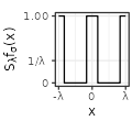
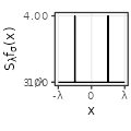
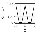
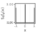
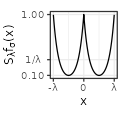
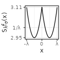
\[S_{\lambda}f_{\sigma}(x) = \frac{1}{\lambda} \mathcal{F}{f_{\sigma}} \left( 0 \right) + \frac{2}{\lambda} \sum_{k=1}^{+\infty} \mathcal{F}{f_{\sigma}} \left( \frac{k}{\lambda} \right) \cos \left( 2\pi \frac{k}{\lambda} x \right),\] \[S_{\lambda}g_{\sigma}(x) = -\frac{4\pi}{\lambda^2} \sum_{k=1}^{+\infty} k \mathcal{F}{f_{\sigma}} \left( \frac{k}{\lambda} \right) \sin \left( 2\pi \frac{k}{\lambda} x \right).\]The following table shows the shape of the summation for a fixed \(\sigma\) as a function of \(\lambda\). The \(x\)-axis is always set on \([-\lambda, \lambda]\) (i.e., two periods), while the \(y\)-axis is adapted to the figure. The last column shows the video for decreasing \(\lambda\). The sum is here always computed with the closed-form expression (proofs are found after the table).
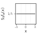
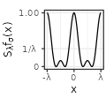
| $$S_{\lambda}f_{\sigma}(x)$$ | $$\lambda=30$$ | $$\lambda=3$$ | $$\lambda=1/3$$ | $$\text{video}$$ |
| Rectangular$$(\sigma=1)$$ | 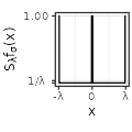 |
 |
 |
|
| Linear$$(\sigma=1)$$ | 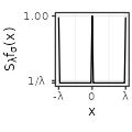 |
 |
 |
|
| Exponential$$(\sigma=1)$$ |  |
 |
 |
|
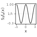
| Polynomial$$(\sigma=1)$$ | 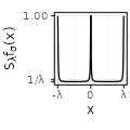 |
 |
 |
|
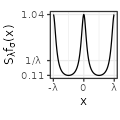
| Gaussian$$(\sigma=1)$$ |  |
 |
 |
|
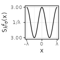
| Sinc$$(\sigma=1)$$ | 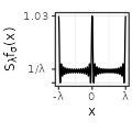 |
 |
 |
|
| Sincsquare$$(\sigma=1)$$ | 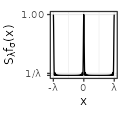 |
 |
 |
For all types, several observations can be made on the function restricted on the interval \([-\lambda/2, \lambda/2)\):
- its integral sums to one by construction, for any positive values of \(\sigma\) and \(\lambda\),
- for \(\lambda\) large, its distribution is almost the same as the initial base function (cf the column with \(\lambda=30\), viewed at a distance on the x-axis),
- for \(\lambda\) tiny, its distribution is almost the same as the uniform distribution (cf the column with \(\lambda=1/3\), viewed at a close range on the y-axis; observe that the whole range is always close to \(1/\lambda\)).
Each type has also specific shapes for the sum \(S_{\lambda}f\). The Rectangular and Linear types have an interesting accelerating oscillating pattern when \(\lambda \rightarrow 0\), while are uniformly distributed almost everywhere for some values of \(\lambda\) (such as \(\lambda = 1/3\) in the table above). The Exponential type stabilizes without oscillations when \(\lambda \rightarrow 0\), while keeping a peak in \(x=0\). The Polynomial and Gaussian types have similar regular shapes for \(\lambda \rightarrow 0\), that look visually extremely close to cosinus. The Sinc and Sincsquare types abruptly change their shapes for specific values of \(\lambda\), and are exactly uniformly distributed for small values of \(\lambda\).
Closed-form expressions
To better understand those patterns, we derive below the closed-form expression of \(S_{\lambda}f_{\sigma}\) and \(S_{\lambda}g_{\sigma}\) for the different types.
We first define the following (\(\tilde{x}\) is used for the Rectangular, Linear, and Exponential types; \(\breve{\sigma}\) is used for the Rectangular type; \(\tilde{\sigma}\) is used for the Linear and Exponential types; \(\Delta\) is used for the Rectangular and Linear types; \(\vartheta_3\) is used for the Gaussian type; \(\left\lfloor z \right\rfloor_{+}\) is used for the Sinc and Sincsquare types):
- \(\tilde{x} \in [-\lambda/2, \lambda/2)\) such that \(x = \tilde{x} + i\lambda\) (\(i\) integer), i.e. \(\tilde{x} := x - \lambda \left\lfloor \frac{x}{\lambda} + \frac{1}{2} \right\rfloor,\)
- \(\breve{\sigma} \in [-\lambda, \lambda)\) such that \(\sigma = \breve{\sigma} + 2i\lambda\) (\(i\) integer), i.e. \(\breve{\sigma} := \sigma - 2 \lambda \left\lfloor \frac{\sigma}{2\lambda} + \frac{1}{2} \right\rfloor,\)
- \(\tilde{\sigma} \in [-\lambda/2, \lambda/2)\) such that \(\sigma = \tilde{\sigma} + i\lambda\) (\(i\) integer), i.e. \(\tilde{\sigma} := \sigma - \lambda \left\lfloor \frac{\sigma}{\lambda} + \frac{1}{2} \right\rfloor.\)
- \(\Delta(x', \sigma') := \mathbf{1}_{(\lvert x' \rvert<\lvert \sigma' \rvert)\text{ or } (\lvert x' \rvert=\lvert \sigma' \rvert \text{ and } \sigma'>0) \text{ or } (x' = 0)}\),
- \(\vartheta_3(z,q) := \sum_{k=-\infty}^{+\infty} q^{k^2} e^{2kiz}\) (for \(z \in \mathbb{R}\) and \(q > 0\)) the Jacobi theta 3 function,
- \(\left\lfloor x \right\rfloor_{+} := \left\lfloor x \right\rfloor + 1\) (which is the ceil function except for \(x\) integer).
The following formulas for \(S_{\lambda}f_{\sigma}(x)\) and \(S_{\lambda}g_{\sigma}(x)\) are defined for \(x \in \mathbb{R}\) and \(\sigma, \lambda > 0\).
For the Rectangular type
\[S_{\lambda}f_{\sigma}(x) = \frac{1}{\lambda} \left( 1 - \frac{\breve{\sigma}}{\sigma} \right) + \Delta(\tilde{x}, \breve{\sigma}/2) \frac{(-1)^{\mathbf{1}_{\breve{\sigma} < 0}}}{\sigma}.\]For the values for which \(S_{\lambda}g_{\sigma}\) is defined (we don’t use distributions here), we deduce:
\[S_{\lambda}g_{\sigma}(x) = 0.\]Proof (click to expand).
Please refer to the Linear case for details. This proof follows the same strategy, using \(\breve{\sigma}\) instead of \(\tilde{\sigma}\), because of the form of the base function. The specific section to look at in the Linear case proof is the computation of \(\frac{1}{\sigma} \left(M^{-}+M^{+}+1 \right)\).
For the Linear type
\[S_{\lambda}f_{\sigma}(x) = \frac{1}{\lambda} \left( 1 - \frac{\tilde{\sigma}^2}{\sigma^2} \right) + \Delta(\tilde{x}, \tilde{\sigma}) \frac{\lvert \tilde{\sigma} \rvert - \lvert \tilde{x} \rvert}{\sigma^2}.\]For the values for which \(S_{\lambda}g_{\sigma}\) is defined, we deduce:
\[S_{\lambda}g_{\sigma}(x) = -\frac{\text{sign}(\tilde{x})}{\sigma^2} \Delta(\tilde{x}, \tilde{\sigma}).\]Proof (click to expand).
Initial computations
The indicator function present in the definition of the base function makes the calculations cumbersome.
Let \(x \in \mathbb{R}\) and \(\sigma, \lambda > 0\). For ease of notation, we define:
\[M^{-}:= \left\lfloor \frac{\sigma + x}{\lambda}\right\rfloor,~M^0 := \left\lfloor \frac{x}{\lambda}\right\rfloor,~M^{+}:= \left\lfloor \frac{\sigma - x}{\lambda}\right\rfloor.\]We let \(I\) the set of integers \(k\) verifying \(|x+k\lambda| \leq \sigma\), i.e. such that \(-M^{-} \leq k \leq M^{+}\). This set is further partitioned into \(I^{-}\) when \(x+k\lambda < 0\), and \(I^{+}\) when \(x+k\lambda \geq 0\). Globally,
- \(I^{-}\) are the elements with \(-M^{-} \leq k \leq -M^0-1\), and
- \(I^{+}\) are the elements with \(-M^0 \leq k \leq M^{+}\).
Any of those three sets can be empty.
The initial formula for \(S_{\lambda}f_{\sigma}(x)\) can be decomposed as follows:
\[\begin{align*} S_{\lambda}f_{\sigma}(x) =& \frac{1}{\sigma} \left[ \sum_{I^{-}} \left( 1 - \frac{-x-k\lambda}{\sigma} \right) + \sum_{I^{+}} \left( 1 - \frac{x+k\lambda}{\sigma} \right) \right] \\ =& \frac{1}{\sigma} \left[ |I| - \frac{1}{\sigma} \left( \sum_{I^{-}} \left( -x-k\lambda \right) + \sum_{I^{+}} \left( x+k\lambda \right) \right) \right] \\ =& \frac{1}{\sigma} |I| - \frac{x}{\sigma^2} \left( -|I^{-}| + |I^{+}| \right) - \frac{\lambda}{\sigma^2} \left( -\sum_{I^{-}} k + \sum_{I^{+}} k \right). \end{align*}\]Using the formula for arithmetic series, we obtain:
\[\begin{align*} S_{\lambda}f_{\sigma}(x) =& \frac{1}{\sigma} |I| - \frac{x}{\sigma^2} \left(|I^{+}|-|I^{-}|\right) \\ -& \frac{\lambda}{2\sigma^2} \left( \left(M^{+}-M^0 \right)|I^{+}| + \left( M^{-}+M^0+1 \right) |I^{-}| \right). \end{align*}\]We have (in all cases, even when the sets are empty):
\[\lvert I^{+} \rvert = M^{+}+M^0+1,~\lvert I^{-} \rvert = -M^0+M^{-},~\lvert I \rvert = M^{+}+M^{-}+1,\]so that:
\[\begin{align*} S_{\lambda}f_{\sigma}(x) =& \frac{1}{\sigma} \left(M^{-}+M^{+}+1 \right) \\ -& \frac{\lambda}{2\sigma^2} \left(M^{+}(M^{+}+1) - 2M^0(M^0+1) + M^{-}(M^{-}+1) \right) \\ -& \frac{x}{\sigma^2} \left(M^{+}-M^{-}+1+2M^0 \right). \end{align*}\]Restriction to the \([-\lambda/2, \lambda/2)\) interval
In all the following we consider \(x \in [-\lambda/2, \lambda/2)\) only (this is enough given the periodicity). We further let \(\tilde{\sigma} \in [-\lambda/2, \lambda/2)\) such that \(\sigma = \tilde{\sigma} + i\lambda\) (for a certain integer \(i\)). We let \(\tilde{M}^{-}:= \left\lfloor \frac{\tilde{\sigma} + x}{\lambda}\right\rfloor\) and \(\tilde{M}^{+}:= \left\lfloor \frac{\tilde{\sigma} - x}{\lambda}\right\rfloor.\) Since both \(\tilde{\sigma}\) and \(x\) are in \([-\lambda/2, \lambda/2)\), all \(\tilde{M}^{-}\), \(\tilde{M}^{0}\), and \(\tilde{M}^{+}\) are in \(\lbrace -1, 0 \rbrace\) (since, before taking the floor function, the values are respectively in \([-1, 1)\), \([-1/2,1/2)\), and \((-1,1)\)). Since \(M^0 \in \lbrace -1, 0\rbrace\), we have \(M^0 = 0\) if and only if \(x \geq 0\).
Term in \(x\)
In this section, we are interested by the following term:
\[S_1 := -\frac{x}{\sigma^2} \left(M^{+}-M^{-}+1+2M^0 \right).\]We observe that \(M^{+}-M^{-} = \tilde{M}^{+}-\tilde{M}^{-}\), so that:
\[S_1 = -\frac{x}{\sigma^2} \left(\tilde{M}^{+}-\tilde{M}^{-}+1-2\mathbf{1}_{x<0} \right).\]There are six cases to consider:
Case 1: In the case of \(x=0\), we have \(S_1=0\).
Case 2: In the case of \(\tilde{\sigma}=0\) and \(x \neq 0\), we have \(\tilde{M}^{-}=-\mathbf{1}_{x<0}\) and \(\tilde{M}^{+}=-\mathbf{1}_{x>0}\), so \(M^{+}-M^{-}+1+2M^0 = -\mathbf{1}_{x>0}-\mathbf{1}_{x<0}+1 = 0\) (since \(x \neq 0\)), and finally \(S_1=0\).
Case 3: In the case of \(\lvert x \rvert< \lvert \tilde{\sigma} \rvert\) and \(\tilde{\sigma} \neq 0\) and \(x \neq 0\), we always obtain \(S_1=-\lvert x \rvert/\sigma^2\).
Case 4: In the case of \(\lvert x \rvert>\lvert \tilde{\sigma} \rvert\) and \(\tilde{\sigma} \neq 0\) and \(x \neq 0\), we always obtain \(S_1=0\).
Case 5: In the case of \(\lvert x \rvert=\lvert \tilde{\sigma} \rvert\) and \(\tilde{\sigma} > 0\), we get \(\tilde{M}^{+}=\tilde{M}^{-}=0\), so \(S_1=-\lvert x \rvert/\sigma^2\).
Case 6: In the case of \(\lvert x \rvert=\lvert \tilde{\sigma} \rvert\) and \(\tilde{\sigma} < 0\), the two sub-cases gives \(S_1=0\).
Merging all the cases, we finally obtain (for \(x \in [-\lambda/2, \lambda/2)\)):
\[S_1 = -\frac{\lvert x \rvert}{\sigma^2} \mathbf{1}_{(\lvert x \rvert<\lvert \tilde{\sigma} \rvert)\text{ or } (\lvert x \rvert=\lvert\tilde{\sigma}\rvert \text{ and } \tilde{\sigma}>0)}.\]Constant terms
In this section, we are interested by the following term:
\[\begin{align*} S_2 :=& \frac{1}{\sigma} \left(M^{-}+M^{+}+1 \right) - \frac{\lambda}{2\sigma^2} \left(M^{+}(M^{+}+1) - 2M^0(M^0+1) + M^{-}(M^{-}+1) \right). \end{align*}\]Since \(M^0(M^0+1)=\tilde{M}^{-}(\tilde{M}^{-}+1)=\tilde{M}^{+}(\tilde{M}^{+}+1)=0\), \(M^{-}=\tilde{M}^{-}+i\), and \(M^{+}=\tilde{M}^{+}+i\), we have:
\[\begin{align*} S_2 =& \frac{1}{\sigma} \left(\tilde{M}^{+} + \tilde{M}^{-}+ 2i +1 \right) - \frac{\lambda}{2\sigma^2} \left(\left(2\tilde{M}^{+}i + i^2 + i\right) + \left(2\tilde{M}^{-}i + i^2+ i\right) \right) \\ =& \frac{1}{\sigma} \left(\tilde{M}^{+} + \tilde{M}^{-}+ 2i +1 \right) -\frac{\lambda i}{\sigma^2} \left(\tilde{M}^{+} + \tilde{M}^{-} + i + 1 \right). \end{align*}\]We next replace the value of \(i=\frac{\sigma - \tilde{\sigma}}{\lambda}\):
\[\begin{align*} S_2 =& \frac{1}{\sigma} \left(\tilde{M}^{+} + \tilde{M}^{-} + 2i +1 \right) -\frac{1}{\sigma} \left(\tilde{M}^{+} + \tilde{M}^{-} + i + 1 \right) +\frac{\tilde{\sigma}}{\sigma^2} \left(\tilde{M}^{+} + \tilde{M}^{-} + i + 1 \right)\\ =& \frac{1}{\lambda} - \frac{\tilde{\sigma}^2}{\lambda\sigma^2} + \frac{\tilde{\sigma}}{\sigma^2} \left(\tilde{M}^{+} + \tilde{M}^{-} + 1 \right). \end{align*}\]We compute \(\tilde{M}^{+} + \tilde{M}^{-} + 1 \in \lbrace -1,0,1 \rbrace\) as in the previous section and obtain:
\[\tilde{M}^{+} + \tilde{M}^{-} + 1 = \mathbf{1}_{(\lvert x \rvert<\lvert \tilde{\sigma} \rvert)\text{ or } (\lvert x \rvert=\lvert\tilde{\sigma}\rvert \text{ and } \tilde{\sigma}>0) \text{ or } (x = 0)} \left( 2 \mathbf{1}_{\tilde{\sigma} \geq 0} -1 \right),\]so finally the constant term is:
\[\begin{align*} S_2 =& \frac{1}{\lambda} - \frac{\tilde{\sigma}^2}{\lambda\sigma^2} + \frac{\lvert \tilde{\sigma} \rvert}{\sigma^2} \mathbf{1}_{(\lvert x \rvert<\lvert \tilde{\sigma} \rvert)\text{ or } (\lvert x \rvert=\lvert\tilde{\sigma}\rvert \text{ and } \tilde{\sigma}>0) \text{ or } (x = 0)}. \end{align*}\]Final form
We let \(\Delta\) the following condition:
\[\Delta := \Delta(x, \tilde{\sigma}) := \mathbf{1}_{(\lvert x \rvert<\lvert \tilde{\sigma} \rvert)\text{ or } (\lvert x \rvert=\lvert\tilde{\sigma}\rvert \text{ and } \tilde{\sigma}>0) \text{ or } (x = 0)}.\]\(S_{\lambda}f_{\sigma}(x)\) is the sum of the terms \(S_1\) and \(S_2\) computed previously:
\[\begin{align*} S_{\lambda}f_{\sigma}(x) =& -\frac{\lvert x \rvert}{\sigma^2} \Delta + \frac{1}{\lambda} - \frac{\tilde{\sigma}^2}{\lambda\sigma^2} + \frac{\lvert \tilde{\sigma} \rvert}{\sigma^2} \Delta \\ =& \frac{1}{\lambda} \left( 1 - \frac{\tilde{\sigma}^2}{\sigma^2} \right) + \Delta \frac{\lvert \tilde{\sigma} \rvert - \lvert x \rvert}{\sigma^2}. \end{align*}\]The form for the derivative is directly deduced.
For the Exponential type
\[S_{\lambda}f_{\sigma}(x) = \frac{1}{\sigma} \frac{\cosh \left( \frac{\lambda}{\sigma} - \frac{2\lvert \tilde{x} \rvert}{\sigma} \right) }{\sinh \left( \frac{\lambda}{\sigma}\right)}.\]For the values for which \(S_{\lambda}g_{\sigma}\) is defined (\(\tilde{x} \neq 0\) in this case), we deduce:
\[S_{\lambda}g_{\sigma}(x) = -\frac{\text{sign}(\tilde{x})}{2} \frac{\sinh \left( \frac{\lambda}{\sigma} - \frac{2\lvert \tilde{x} \rvert}{\sigma} \right)}{\sinh \left( \frac{\lambda}{\sigma}\right)}.\]Proof (click to expand).
Let \(x \in \mathbb{R}\) and \(\sigma, \lambda > 0\). As for the linear case, we define \(M^0 := \left\lfloor \frac{x}{\lambda}\right\rfloor\).
The sum \(S_{\lambda}f_{\sigma}(x)\) can be written:
\[\begin{align*} S_{\lambda}f_{\sigma}(x) =& \frac{1}{\sigma} \left[ \sum_{k=-\infty}^{-M^0-1} e^{2\frac{x+k\lambda}{\sigma}} + \sum_{k=-M^0}^{+\infty} e^{2\frac{-x-k\lambda}{\sigma}} \right] \\ =& \frac{1}{\sigma} \left[ e^{\frac{2x}{\sigma}} \frac{-e^{-\frac{2\lambda M^0}{\sigma}}}{1 - e^{\frac{2\lambda}{\sigma}}} + e^{-\frac{2x}{\sigma}} \frac{e^{\frac{2\lambda M^0}{\sigma}}}{1 - e^{\frac{-2\lambda}{\sigma}}} \right]. \end{align*}\]Restricting on \(x \in [0, \lambda/2]\), we have \(M^0=0\), so on this interval:
\[S_{\lambda}f_{\sigma}(x) = \frac{1}{\sigma} \left[ - \frac{e^{\frac{2x}{\sigma}}}{1 - e^{\frac{2\lambda}{\sigma}}} + \frac{e^{-\frac{2x}{\sigma}}}{1 - e^{\frac{-2\lambda}{\sigma}}} \right]\]Since the function is even, we deduce for \(x \in [-\lambda/2, \lambda/2)\):
\[S_{\lambda}f_{\sigma}(x) = \frac{1}{\sigma} \left[-\frac{e^{\frac{2\lvert x \rvert}{\sigma}}}{1 - e^{\frac{2\lambda}{\sigma}}} + \frac{e^{-\frac{2\lvert x \rvert}{\sigma}}}{1 - e^{-\frac{2\lambda}{\sigma}}} \right],\]which is extended on the whole real line using \(\tilde{x}\). By multiplying the first term by \(\frac{e^{-\frac{\lambda}{\sigma}}}{e^{-\frac{\lambda}{\sigma}}}\) and the second term by \(\frac{e^{\frac{\lambda}{\sigma}}}{e^{\frac{\lambda}{\sigma}}}\), we deduce:
\[S_{\lambda}f_{\sigma}(x) = \frac{1}{\sigma} \frac{\cosh \left( \frac{\lambda}{\sigma} - \frac{2\lvert \tilde{x} \rvert}{\sigma} \right) }{\sinh \left( \frac{\lambda}{\sigma}\right)}.\]By taking the derivative, we finally obtain:
\[S_{\lambda}g_{\sigma}(x) = \frac{-\text{sign}(\tilde{x})}{2} \frac{\sinh \left( \frac{\lambda}{\sigma} - \frac{2 \lvert \tilde{x} \rvert}{\sigma} \right)}{\sinh \left( \frac{\lambda}{\sigma}\right)}.\]For the Polynomial type
\[S_{\lambda}f_{\sigma}(x) = \frac{1}{\lambda} \frac{\sinh \left( \frac{2 \sigma}{\lambda} \right)}{\cosh \left( \frac{2 \sigma}{\lambda} \right)-\cos \left( \frac{2\pi x}{\lambda} \right)},\] \[S_{\lambda}g_{\sigma}(x) = - \frac{2 \pi}{\lambda^2} \frac{\sinh \left( \frac{2 \sigma}{\lambda} \right) \sin \left( \frac{2\pi x}{\lambda} \right)}{\left( \cosh \left( \frac{2 \sigma}{\lambda} \right) - \cos \left( \frac{2\pi x}{\lambda} \right) \right)^2}.\]Proof (click to expand).
Using the Poisson summation formula, we have for \(x \in \mathbb{R}\), with \(A:=\frac{2\pi x}{\lambda}\) and \(B:= \frac{2 \sigma}{\lambda}\):
\[\begin{align*} S_{\lambda}f_{\sigma}(x) =& \frac{1}{\lambda} \sum_{k=-\infty}^{+\infty} e^{- \lvert k \rvert B} e^{ikA}\\ =& \frac{1}{\lambda} \left[ \sum_{k=1}^{+\infty} \left( e^{-B-iA} \right)^k + \sum_{k=1}^{+\infty} \left( e^{-B+iA} \right)^k + 1 \right] \\ =& \frac{1}{\lambda} \left[ \frac{e^{-B-iA}}{1 - e^{-B-iA}} + \frac{e^{-B+iA}}{1 - e^{-B+iA}} + 1 \right] \\ =& \frac{1}{\lambda} \left[ \frac{(1 - e^{-B+iA})e^{-B-iA} + (1 - e^{-B-iA})e^{-B+iA}}{(1 - e^{-B-iA})(1 - e^{-B+iA})} + 1 \right] \\ =& \frac{1}{\lambda} \left[ \frac{e^{-B-iA} + e^{-B+iA} - 2e^{-2B}}{1 - e^{-B-iA}-e^{-B+iA}+e^{-2B}} + 1 \right] \\ =& \frac{1}{\lambda} \left[ \frac{e^{-iA} + e^{+iA} - 2e^{-B}}{e^B - e^{-iA}-e^{+iA}+e^{-B}} + \frac{e^B - e^{-iA}-e^{+iA}+e^{-B}}{e^B - e^{-iA}-e^{+iA}+e^{-B}} \right] \\ =& \frac{1}{\lambda} \frac{e^B-e^{-B}}{e^B+e^{-B}-e^{iA}-e^{-iA}} \\ =& \frac{1}{\lambda} \frac{\sinh(B)}{\cosh(B)-\cos(A)} \\ \end{align*}\]The derivative can be deduced easily.
For the Gaussian type
\[S_{\lambda}f_{\sigma}(x) = \frac{1}{\lambda} \vartheta_3 \left( \frac{\pi x}{\lambda}, e^{-\frac{\pi \sigma^2}{\lambda^2}} \right),\] \[S_{\lambda}g_{\sigma}(x) = \frac{\pi}{\lambda^2} \vartheta_3' \left( \frac{\pi x}{\lambda}, e^{-\frac{\pi \sigma^2}{\lambda^2}} \right).\]Proof (click to expand).
Using the Poisson summation formula, we have for \(x \in \mathbb{R}\), with \(z:=\frac{\pi x}{\lambda}\) and \(q:= e^{-\frac{\pi\sigma^2}{\lambda^2}}\) (in particular \(q>0\)):
\[\begin{align*} S_{\lambda}f_{\sigma}(x) =& \frac{1}{\lambda} + \frac{2}{\lambda} \sum_{k=1}^{+\infty} e^{-\pi \sigma^2 \frac{k^2}{\lambda^2}} \cos \left( 2\pi \frac{k}{\lambda} x \right)\\ =& \frac{1}{\lambda} + \frac{2}{\lambda} \sum_{k=1}^{+\infty} q^{k^2} \cos \left( 2kz \right) \\ =& \frac{1}{\lambda} \sum_{k=-\infty}^{+\infty} q^{k^2} e^{2kiz} \\ =& \frac{1}{\lambda} \vartheta_3(z,q).\\ \end{align*}\]The derivative in \(z\) of the Jacobi theta 3 function is given by:
\[\vartheta_3'(z,q) = -4 \sum_{k=1}^{+\infty} k q^{k^2} \sin \left( 2kz \right),\]and the derivative in \(x\) of \(S_{\lambda}f_{\sigma}(x)\) is:
\[S_{\lambda}g_{\sigma}(x) = \frac{\pi}{\lambda^2} \vartheta_3' \left( \frac{\pi x}{\lambda}, e^{-\frac{\pi \sigma^2}{\lambda^2}} \right).\]For the Sinc type
\[S_{\lambda}f_{\sigma}(x) = \frac{1}{\lambda \sin \left( \frac{\pi x}{\lambda} \right)} \sin \left( \left( 2 \left\lfloor\frac{\lambda}{2\sigma}\right\rfloor + 1\right) \frac{\pi x}{\lambda} \right),\] \[S_{\lambda}g_{\sigma}(x) = -\frac{\pi}{\lambda^2 \sin^2 \left( \frac{\pi x}{\lambda} \right)} \left[ \left\lfloor\frac{\lambda}{2\sigma}\right\rfloor_{+} \sin \left( \left\lfloor\frac{\lambda}{2\sigma}\right\rfloor \frac{2\pi x}{\lambda} \right) - \left\lfloor\frac{\lambda}{2\sigma}\right\rfloor \sin \left( \left\lfloor\frac{\lambda}{2\sigma}\right\rfloor_{+} \frac{2\pi x}{\lambda} \right) \right].\]Note that those functions are extended by continuity for all undefined \(x\), e.g. in \(x=0\).
Proof (click to expand).
Using the Poisson summation formula, we have for \(x \neq \lambda n\) (this case can be directly done separately):
\[\begin{align*} S_{\lambda}f_{\sigma}(x) =& \frac{1}{\lambda} + \frac{2}{\lambda} \sum_{k=1}^{+\infty} \mathbf{1}_{\frac{k}{\lambda} \in \left[ -\frac{1}{2 \sigma}, \frac{1}{2 \sigma} \right]} \cos \left( 2\pi \frac{k}{\lambda} x \right)\\ =& \frac{1}{\lambda} + \frac{2}{\lambda} \sum_{k=1}^{\left\lfloor\frac{\lambda}{2\sigma}\right\rfloor} \cos \left( 2\pi \frac{k}{\lambda} x \right) \\ =& \frac{1}{\lambda} + \frac{2}{\lambda} \frac{1}{2} \left[ -1 + \frac{\sin \left( \left( 2 \left\lfloor\frac{\lambda}{2\sigma}\right\rfloor + 1\right) \frac{\pi x}{\lambda} \right) }{\sin \left( \frac{\pi x}{\lambda} \right)} \right] \\ =& \frac{1}{\lambda} \frac{\sin \left( \left( 2 \left\lfloor\frac{\lambda}{2\sigma}\right\rfloor + 1\right) \frac{\pi x}{\lambda} \right) }{\sin \left( \frac{\pi x}{\lambda} \right)}. \end{align*}\]Defining \(A:=\frac{\pi}{\lambda}\) and \(B:=2 \left\lfloor\frac{\lambda}{2\sigma}\right\rfloor + 1\),
\[\begin{align*} S_{\lambda}f_{\sigma}(x)= \frac{1}{\lambda} \frac{\sin \left( ABx \right) }{\sin \left( Ax\right)}, \end{align*}\]so by taking the derivate, we obtain:
\[\begin{align*} S_{\lambda}g_{\sigma}(x) =& \frac{A}{\lambda \sin^2 \left( Ax \right)} \left[ B \cos \left( ABx \right) \sin \left( Ax \right) - \sin \left( ABx \right) \cos \left( Ax \right) \right]. \end{align*}\]We further use the identity:
\[B \cos(ABx)\sin(Ax) - \sin(ABx)\cos(Ax) = \frac{1}{2} \left[ (B-1) \sin(A(B+1)x) - (B+1) \sin (A(B-1)x) \right]\]to derive:
\[\begin{align*} S_{\lambda}g_{\sigma}(x) =& \frac{A}{2 \lambda \sin^2 \left( Ax \right)} \left[ (B-1) \sin(A(B+1)x) - (B+1) \sin (A(B-1)x) \right]\\ =& \frac{A}{\lambda \sin^2 \left( Ax \right)} \left[ \left\lfloor\frac{\lambda}{2\sigma}\right\rfloor \sin(A(B+1)x) - \left( \left\lfloor\frac{\lambda}{2\sigma}\right\rfloor + 1 \right) \sin (A(B-1)x) \right] \\ =& \frac{\pi}{\lambda^2 \sin^2 \left( \frac{\pi x}{\lambda} \right)} \left[ \left\lfloor\frac{\lambda}{2\sigma}\right\rfloor \sin \left( \left( \left\lfloor\frac{\lambda}{2\sigma}\right\rfloor + 1 \right) \frac{2\pi x}{\lambda} \right) - \left( \left\lfloor\frac{\lambda}{2\sigma}\right\rfloor + 1 \right) \sin \left( \left\lfloor\frac{\lambda}{2\sigma}\right\rfloor \frac{2\pi x}{\lambda} \right) \right]. \end{align*}\]For the Sincsquare type
\[\begin{align*} S_{\lambda}f_{\sigma}(x) =& \frac{1}{\lambda \sin \left( \frac{\pi x}{\lambda} \right)} \sin \left( \left( 2 \left\lfloor\frac{\lambda}{\sigma}\right\rfloor + 1\right) \frac{\pi x}{\lambda} \right) \\ -& \frac{\sigma}{2\lambda^2 \sin^2 \left( \frac{\pi x}{\lambda} \right)} \left( \left\lfloor\frac{\lambda}{\sigma}\right\rfloor_{+} \cos \left( \left\lfloor\frac{\lambda}{\sigma}\right\rfloor \frac{2 \pi x}{\lambda} \right) - \left\lfloor\frac{\lambda}{\sigma}\right\rfloor \cos \left( \left\lfloor\frac{\lambda}{\sigma}\right\rfloor_{+} \frac{2 \pi x}{\lambda} \right) - 1 \right). \end{align*}\]For the derivative, we first define:
\[D_c := \cos \left( \left\lfloor\frac{\lambda}{\sigma}\right\rfloor \frac{2 \pi x}{\lambda} \right) + \left\lfloor\frac{\lambda}{\sigma}\right\rfloor \left( \cos \left( \left\lfloor\frac{\lambda}{\sigma}\right\rfloor \frac{2 \pi x}{\lambda} \right)- \cos \left( \left\lfloor\frac{\lambda}{\sigma}\right\rfloor_{+} \frac{2 \pi x}{\lambda} \right) \right) - 1,\] \[D_s := \left\lfloor\frac{\lambda}{\sigma}\right\rfloor_{+} \left\lfloor\frac{\lambda}{\sigma}\right\rfloor \left( \sin \left( \left\lfloor\frac{\lambda}{\sigma}\right\rfloor \frac{2 \pi x}{\lambda} \right)- \sin \left( \left\lfloor\frac{\lambda}{\sigma}\right\rfloor_{+} \frac{2 \pi x}{\lambda} \right) \right),\]and we have:
\[\begin{align*} S_{\lambda}g_{\sigma}(x) =& -\frac{\pi}{\lambda^2 \sin^2 \left( \frac{\pi x}{\lambda}\right)} \left[ \left\lfloor\frac{\lambda}{\sigma}\right\rfloor_{+} \sin \left( \left\lfloor\frac{\lambda}{\sigma}\right\rfloor \frac{2 \pi x}{\lambda} \right) - \left\lfloor\frac{\lambda}{\sigma}\right\rfloor \sin \left( \left\lfloor\frac{\lambda}{\sigma}\right\rfloor_{+} \frac{2 \pi x}{\lambda} \right) \right]\\ &+ \frac{\pi \sigma}{\lambda^3 \sin^3 \left( \frac{\pi x}{\lambda} \right)} \left[ \cos \left( \frac{\pi x}{\lambda} \right) D_c + \sin \left( \frac{\pi x}{\lambda} \right) D_s \right]. \end{align*}\]Note that those functions are extended by continuity for all undefined \(x\), e.g. in \(x=0\), as for the Sinc type.
Proof (click to expand).
Using the Poisson summation formula, we have for \(x \neq \lambda n\) (this case can be directly done separately):
\[\begin{align*} S_{\lambda}f_{\sigma}(x) =& \frac{1}{\lambda} + \frac{2}{\lambda} \sum_{k=1}^{+\infty} \left( 1 - \frac{k}{\lambda} \sigma \right) \mathbf{1}_{\frac{k}{\lambda} \leq \frac{1}{\sigma}} \cos \left( 2\pi \frac{k}{\lambda} x \right)\\ =& \frac{1}{\lambda} + \frac{2}{\lambda} \sum_{k=1}^{\left\lfloor\frac{\lambda}{\sigma}\right\rfloor} \left( 1 - \frac{k \sigma}{\lambda} \right) \cos \left( 2\pi \frac{k}{\lambda} x \right) \\ =& \frac{1}{\lambda} + \frac{2}{\lambda} \sum_{k=1}^{\left\lfloor\frac{\lambda}{\sigma}\right\rfloor} \cos \left( 2\pi \frac{k}{\lambda} x \right) - \frac{2\sigma}{\lambda^2} \sum_{k=1}^{\left\lfloor\frac{\lambda}{\sigma}\right\rfloor} k \cos \left( 2\pi \frac{k}{\lambda} x \right). \end{align*}\]The two first terms correspond to the Sinc case above with \(\sigma/2\), while the other term is a classical sum. With \(N:=\left\lfloor\frac{\lambda}{\sigma}\right\rfloor\) and \(A := 2 \pi x / \lambda\), we obtain:
\[\begin{align*} S_{\lambda}f_{\sigma}(x) =& \left[ \frac{1}{\lambda \sin \left( A/2 \right)} \sin \left( \left( 2 N + 1\right) A/2 \right) \right] - \frac{2\sigma}{\lambda^2} \sum_{k=1}^{N} k \cos \left( Ak\right)\\ =& \left[ \frac{1}{\lambda \sin \left( A/2 \right)} \sin \left( \left( 2 N + 1\right) A/2 \right) \right] - \frac{2\sigma}{\lambda^2} \frac{1}{4 \sin^2 \left(A/2 \right)} \left( \left(N + 1\right) \cos \left(N A \right) - N \cos \left( \left(N+1 \right) A \right) -1 \right) \\ =& \frac{1}{\lambda \sin \left( A/2 \right)} \sin \left( \left( 2 N + 1\right) A/2 \right) - \frac{\sigma}{2\lambda^2 \sin^2 \left(A/2 \right)} \left( (N+1) \cos \left( N A \right) - N \cos \left( \left(N+1 \right) A \right) - 1 \right). \end{align*}\]The derivative is then obtained term by term.
Dynamics
We are interested in the dynamics of \(S_{\lambda}f_{\sigma}\) when \(\lambda \to 0\) (with \(\sigma > 0\) assumed to be fixed).
To simplify and gain a deeper comprehension of the closed-form expressions, we perform the following normalizations:
- the sum is normalized using the shift \(1 / \lambda\), that is common for all types, and a scaling term \(N(\lambda, \sigma)\) that changes from type to type,
- the time is defined by \(t := \sigma/\lambda\),
- the space is scaled with: \(z := x/ \lambda\).
The normalized sum is given, as a function of \(t > 0\) and \(z \in \mathbb{R}\), by:
\[Z_t f_{\sigma}(z) := N(\lambda, \sigma) \left( S_{\lambda}f_{\sigma}(x) - \frac{1}{\lambda} \right).\]As before, we explore the different types separately.
For the rest of the section, we define:
- \(\lbrace t \rbrace \in [0, 1)\) the fractional part, i.e. \(\lbrace t \rbrace := t - \left\lfloor t \right\rfloor\),
- \(\lbrace t \rbrace_{-} \in [-1/2, 1/2)\) the shifted fractional part, i.e. \(\lbrace t \rbrace_{-} := t - \left\lfloor t + \frac{1}{2} \right\rfloor\),
- \(\mathbf{\Lambda}(t, z) := \mathbf{1}_{(\lvert t - 1/2 \rvert + \lvert z \rvert< 1/2)\text{ or } (\lvert t - 1/2 \rvert + \lvert z \rvert = 1/2 \text{ and } t < 1/2)}\),
- \(\mathbf{\Delta}(t, z) := \mathbf{1}_{\lvert t - 1/2 \rvert + \lvert z \rvert \leq 1/2}\).
The following formulas for \(Z_t f_{\sigma}(z)\) are defined for \(t > 0\) and \(z \in \mathbb{R}\).
For the Rectangular type
Using the normalization \(N(\lambda, \sigma) = \sigma\), we have:
\[\begin{align*} Z_t f_{\sigma}(z) = \left( 1-2 \lbrace t/2 \rbrace \right) + \left(1-\mathbf{\Lambda}(\lbrace t/2 \rbrace, \lbrace z \rbrace_{-})\right) (-1)^{\mathbf{1}_{\lbrace t/2 \rbrace < 1/2}}. \end{align*}\]Proof (click to expand).
For \(\lambda > 0\), we consider \(x \in [-\lambda/2, \lambda/2)\), or equivalently \(z \in [-1/2, 1/2)\). The closed-form expression for the rectangular type verifies:
\[S_{\lambda}f_{\sigma}(x) - \frac{1}{\lambda} = - \frac{\breve{\sigma}}{\lambda\sigma} + \Delta(x, \breve{\sigma}/2) \frac{(-1)^{\mathbf{1}_{\breve{\sigma}/\lambda < 0}}}{\sigma}.\]Using the normalization: \(N(\lambda, \sigma) = \sigma\), and since \(\breve{\sigma}/\lambda = t - 2 \left\lfloor \frac{t}{2} + \frac{1}{2} \right\rfloor\), we obtain:
\[\begin{align*} Z_t f_{\sigma}(z) =& - \breve{\sigma}/\lambda + \Delta(x, \breve{\sigma}/2) (-1)^{\mathbf{1}_{\breve{\sigma} < 0}} \\ =& -t + 2 \left\lfloor t/2 + 1/2 \right\rfloor + \Delta(x, \breve{\sigma}/2) (-1)^{\mathbf{1}_{t - 2 \left\lfloor t/2 + 1/2 \right\rfloor < 0}}. \end{align*}\]Case when \(t \in (0, 1) \cup [2, 3) \cup [4, 5) \cup \ldots\)
In this case, we have \(t - 2 \left\lfloor t/2+1/2 \right\rfloor = 2 \lbrace t/2 \rbrace\) and:
\[\begin{align*} Z_t f_{\sigma}(z) =& -2 \lbrace t/2 \rbrace + \Delta(x, \breve{\sigma}/2) (-1)^{\mathbf{1}_{2 \lbrace t/2 \rbrace < 0}} \\ =& -2 \lbrace t/2 \rbrace + \Delta(x, \breve{\sigma}/2). \end{align*}\]Case when \(t \in [1, 2) \cup [3, 4) \cup [5, 6) \cup \ldots\)
In this case, we have \(t - 2 \left\lfloor t/2+1/2 \right\rfloor = 2 \lbrace t/2 \rbrace - 2\) and:
\[\begin{align*} Z_t f_{\sigma}(z) =& -2 \lbrace t/2 \rbrace + 2 + \Delta(x, \breve{\sigma}/2) (-1)^{\mathbf{1}_{2 \lbrace t/2 \rbrace - 2 < 0}} \\ =& -2 \lbrace t/2 \rbrace + 2 - \Delta(x, \breve{\sigma}/2). \end{align*}\]In all cases, we obtain:
\[\begin{align*} Z_t f_{\sigma}(z) =& \begin{cases} -2 \lbrace t/2 \rbrace + 1 & \text{if } \Delta(x, \breve{\sigma}/2)=1\\ -2 \lbrace t/2 \rbrace + 2 \mathbf{1}_{\lbrace t/2 \rbrace \geq 1/2} & \text{otherwise}. \end{cases} \end{align*}\]Simplification of \(\Delta\)
From the original definition of \(\Delta\), by dividing each element of the condition by \(\lambda\), using that \(\breve{\sigma}/(2\lambda) = t/2 - \left\lfloor t/2 + 1/2 \right\rfloor\), and \(\lvert t/2 - \left\lfloor t/2 + 1/2 \right\rfloor \rvert = 1/2 - \lvert \lbrace t/2 \rbrace - 1/2 \rvert\), we obtain:
\[\begin{align*} \Delta(x, \breve{\sigma}/2) =& \mathbf{1}_{(\lvert x \rvert<\lvert \breve{\sigma}/2 \rvert)\text{ or } (\lvert x \rvert=\lvert \breve{\sigma}/2 \rvert \text{ and } \breve{\sigma}/2 >0) \text{ or } (x = 0)}\\ =& \mathbf{1}_{(\lvert z \rvert<\lvert \breve{\sigma}/(2\lambda) \rvert)\text{ or } (\lvert z \rvert=\lvert \breve{\sigma}/(2\lambda) \rvert \text{ and } \breve{\sigma}/(2\lambda) >0) \text{ or } (z = 0)} \\ =& \mathbf{1}_{(\lvert z \rvert< 1/2 - \lvert \lbrace t/2 \rbrace - 1/2 \rvert)\text{ or } (\lvert z \rvert=1/2 - \lvert \lbrace t/2 \rbrace - 1/2 \rvert \text{ and } t/2 - \left\lfloor t/2 + 1/2 \right\rfloor >0) \text{ or } (z = 0)} \\ =& \mathbf{1}_{(\lvert z \rvert + \lvert \lbrace t/2 \rbrace - 1/2 \rvert < 1/2)\text{ or } (\lvert z \rvert + \lvert \lbrace t/2 \rbrace - 1/2 \rvert =1/2 \text{ and } t/2 - \left\lfloor t/2 + 1/2 \right\rfloor >0) \text{ or } (z = 0)} \\ =& \mathbf{1}_{(\lvert z \rvert + \lvert \lbrace t/2 \rbrace - 1/2 \rvert < 1/2)\text{ or } (\lvert z \rvert + \lvert \lbrace t/2 \rbrace - 1/2 \rvert =1/2 \text{ and } t/2 - \left\lfloor t/2 + 1/2 \right\rfloor \geq 0)} \\ =& \mathbf{1}_{(\lvert z \rvert + \lvert \lbrace t/2 \rbrace - 1/2 \rvert < 1/2)\text{ or } (\lvert z \rvert + \lvert \lbrace t/2 \rbrace - 1/2 \rvert =1/2 \text{ and } \lbrace t/2 \rbrace < 1/2)} \end{align*}\]We let \(\mathbf{\Lambda}(t, z) := \mathbf{1}_{(\lvert t - 1/2 \rvert + \lvert z \rvert< 1/2)\text{ or } (\lvert t - 1/2 \rvert + \lvert z \rvert = 1/2 \text{ and } t < 1/2)}\).
Final form
\[\begin{align*} Z_t f_{\sigma}(z) =& -2 \lbrace t/2 \rbrace + \mathbf{\Lambda}(\lbrace t/2 \rbrace, z) + 2 (1-\mathbf{\Lambda}(\lbrace t/2 \rbrace, z)) \mathbf{1}_{\lbrace t/2 \rbrace \geq 1/2}\\ =& \left( 1-2 \lbrace t/2 \rbrace \right) + \left( \mathbf{\Lambda}(\lbrace t/2 \rbrace, z) + 2 (1-\mathbf{\Lambda}(\lbrace t/2 \rbrace, z)) \mathbf{1}_{\lbrace t/2 \rbrace \geq 1/2} - 1 \right) \\ =& \left( 1-2 \lbrace t/2 \rbrace \right) + \left(1-\mathbf{\Lambda}(\lbrace t/2 \rbrace, z)\right) (-1)^{\mathbf{1}_{\lbrace t/2 \rbrace < 1/2}}. \end{align*}\]We observe that under this form, the normalized sum \(Z_t f_{\sigma}(z)\) does not depend on \(\sigma\) (given \(t\) and \(z\)). The function is also \(2\)-periodic in time and \(1\)-periodic in space.
Restricting on the single period \(z \in [-1/2, 1/2)\), we observe in the following video:
- (left) the mapping \(z \mapsto Z_t f_{\sigma}(z)\) over time, with marked points for \(z=-1/2\) (blue), \(z=\pm 1/4\) (green), \(z=\pm 1/8\) (yellow) and \(z=0\) (gray); we observe a decreasing motion driven by \(t \mapsto 1-t\), with two separate and symmetric phases before and after \(t=1\),
- (center) the mapping \(\lbrace t \rbrace \mapsto Z_t f_{\sigma}(z)\) for the \(6\) previous marked points over time; we observe that the marked points jump over the three curves \(t \mapsto 2-t\), \(t \mapsto 1-t\), and \(t \mapsto -t\),
- (right) the condition \((t, z) \mapsto \mathbf{\Lambda}(t/2, z)\) represented by a gray square (that in also \(1\)-periodic in space and \(2\)-periodic in time), with the marked points and the space segment \([-1/2, 1/2)\) over time; we observe as expected a change in the behavior of each marked point when entering or leaving the gray zone. On this figure, the numbers correspond to the whole right term of the \(Z_t f_{\sigma}(z)\) formula above. The value is \(0\) inside the gray zone, including the whole axis \(z=0\) but excluding the border for \(2 \lbrace t/2 \rbrace \geq 1\). The value is \(1\) outside the zone for \(2 \lbrace t/2 \rbrace \geq 1\). The value is \(-1\) outside the zone for \(2 \lbrace t/2 \rbrace < 1\). Note that we always have \(2 \lbrace t/2 \rbrace \in [0,2)\).
Additional videos of the mapping \(t \mapsto Z_t f_{\sigma}(z)\) over space, and of the unnormalized mapping \(x \mapsto S_{\lambda}f_{\sigma}(x)\) over time are provided by expanding the following tab.
Additional videos (click to expand).
- Mapping \(t \mapsto Z_t f_{\sigma}(z)\) over space. Note that the colors of this video are not linked with the colors of the previous video.
- Mapping \(x \mapsto S_{\lambda}f_{\sigma}(x)\) over time. In this unnormalized form, we observe as expected a shape equivalent to \(z \mapsto Z_t f_{\sigma}(z)\) over time. The range of the figure is constant and equal to \(2/\sigma\).
For the Linear type
Using the normalization \(N(\lambda, \sigma) = \sigma^2 / \lambda = \sigma t\), we have:
\[\begin{align*} Z_t f_{\sigma}(z) =& \begin{cases} -\lbrace t \rbrace \left( \lbrace t \rbrace - 1 \right) - \lvert \lbrace z \rbrace_{-} \rvert & \text{if } \mathbf{\Delta}(\lbrace t \rbrace, \lbrace z \rbrace_{-})=1\\ -\lbrace t \rbrace^{2}_{-} & \text{otherwise} \end{cases} \\ =& - \min \left( \lbrace t \rbrace \left( \lbrace t \rbrace - 1 \right) + \lvert \lbrace z \rbrace_{-} \rvert, \lbrace t \rbrace^{2}_{-} \right). \end{align*}\]Proof (click to expand).
For \(\lambda > 0\), we consider \(x \in [-\lambda/2, \lambda/2)\), or equivalently \(z \in [-1/2, 1/2)\). The closed-form expression for the linear type verifies:
\[\begin{align*} S_{\lambda}f_{\sigma}(x) - \frac{1}{\lambda} = -\frac{1}{\lambda} \left( 1 - \frac{\lambda}{\sigma} \left\lfloor \frac{\sigma}{\lambda} + \frac{1}{2} \right\rfloor \right)^2 + \Delta(x, \tilde{\sigma}) \left( \left\lvert \sigma^{-1} - \frac{\lambda}{\sigma^2} \left\lfloor \frac{\sigma}{\lambda} + \frac{1}{2} \right\rfloor \right\rvert - \frac{\lvert x \rvert}{\sigma^2} \right). \end{align*}\]Using the normalization: \(N(\lambda, \sigma) = \frac{\sigma^2}{\lambda}\), we obtain:
\[\begin{align*} Z_t f_{\sigma}(z) =& -\frac{\sigma^2}{\lambda^2} \left( 1 - \frac{\lambda}{\sigma} \left\lfloor \frac{\sigma}{\lambda} + \frac{1}{2} \right\rfloor \right)^2 + \Delta(x, \tilde{\sigma}) \left( \left\lvert \frac{\sigma}{\lambda} - \left\lfloor \frac{\sigma}{\lambda} + \frac{1}{2} \right\rfloor \right\rvert - \frac{\lvert x \rvert}{\lambda} \right) \\ =& -t^2 \left( 1 - \frac{1}{t} \left\lfloor t + \frac{1}{2} \right\rfloor \right)^2 + \Delta(x, \tilde{\sigma}) \left( \left\lvert t - \left\lfloor t + \frac{1}{2} \right\rfloor \right\rvert - \lvert z \rvert \right). \end{align*}\]Form depending whether the condition \(\Delta\) is fulfilled or not
When the condition \(\Delta\) is not fulfilled:
\[\begin{align*} Z_t f_{\sigma}(z) = -t^2 \left( 1 - \frac{1}{t} \left\lfloor t + \frac{1}{2} \right\rfloor \right)^2 = - \left(t - \left\lfloor t + \frac{1}{2} \right\rfloor \right)^2 = - \lbrace t \rbrace^{2}_{-}. \end{align*}\]When the condition \(\Delta\) is fulfilled:
\[\begin{align*} Z_t f_{\sigma}(z) =& - \left( t^2 - 2 t \left\lfloor t + \frac{1}{2} \right\rfloor+ \left\lfloor t + \frac{1}{2} \right\rfloor^2 \right) + \left\lvert t - \left\lfloor t + \frac{1}{2} \right\rfloor \right\rvert - \lvert z \rvert \end{align*}\]We further separate in two cases. Either \(t \in (0, 1/2] \cup [1, 3/2] \cup \ldots\), and on those intervals, we have \(t - \left\lfloor t + \frac{1}{2} \right\rfloor \geq 0\) and \(\left\lfloor t + \frac{1}{2} \right\rfloor = \left\lfloor t \right\rfloor\). Otherwise, for \(t \in [1/2, 1] \cup [3/2, 2] \cup \ldots\), we have \(t - \left\lfloor t + \frac{1}{2} \right\rfloor \leq 0\), and \(\left\lfloor t + \frac{1}{2} \right\rfloor = \left\lfloor t \right\rfloor + 1\). In both cases, we obtain (when the condition \(\Delta\) is fulfilled):
\[\begin{align*} Z_t f_{\sigma}(z) = - \left( t - \left\lfloor t \right\rfloor \right) \left( t-\left\lfloor t \right\rfloor-1 \right) - \lvert z \rvert = - \lbrace t \rbrace \left( \lbrace t \rbrace - 1 \right) - \lvert z \rvert. \end{align*}\]Condition \(\Delta\) as a function of \(t\) and \(z\)
From the original definition of \(\Delta\), by dividing each element of the condition by \(\lambda\), and further using that (*):
\[\lvert t - \left\lfloor t + 1/2 \right\rfloor \rvert = 1/2 - \lvert t - \left\lfloor t \right\rfloor - 1/2 \rvert = 1/2 - \lvert \lbrace t \rbrace - 1/2 \rvert,\]we obtain:
\[\begin{align*} \Delta(x, \tilde{\sigma}) =& \mathbf{1}_{(\lvert x \rvert<\lvert \tilde{\sigma} \rvert)\text{ or } (\lvert x \rvert=\lvert \tilde{\sigma} \rvert \text{ and } \tilde{\sigma} >0) \text{ or } (x = 0)} \\ =& \mathbf{1}_{(\lvert z \rvert<\lvert t - \left\lfloor t + 1/2 \right\rfloor \rvert)\text{ or } (\lvert z \rvert=\lvert t - \left\lfloor t + 1/2 \right\rfloor \rvert \text{ and } t - \left\lfloor t + 1/2 \right\rfloor >0) \text{ or } (z = 0)} \\ =& \mathbf{1}_{(\lvert z \rvert< 1/2 - \lvert \lbrace t \rbrace - 1/2 \rvert )\text{ or } (\lvert z \rvert= 1/2 - \lvert \lbrace t \rbrace - 1/2 \rvert \text{ and } t - \left\lfloor t + 1/2 \right\rfloor >0) \text{ or } (z = 0)}. \end{align*}\]We let \(\mathbf{\Delta}(t, z) := \mathbf{1}_{\lvert t - 1/2 \rvert + \lvert z \rvert \leq 1/2}.\) We have \(\mathbf{\Delta}(\lbrace t \rbrace, z) = \Delta(x, \tilde{\sigma})\) when \(\lvert t - 1/2 \rvert + \lvert z \rvert < 1/2\). There is also equality when \(z = 0\). In the remaining case where \(\lvert t - 1/2 \rvert + \lvert z \rvert = 1/2\), we may have \(\mathbf{\Delta}(\lbrace t \rbrace, z) \neq \Delta(x, \tilde{\sigma})\), but in this case the term that is multiplied by \(\Delta\) is always null, since in that case \(\left\lvert t - \left\lfloor t + \frac{1}{2} \right\rfloor \right\rvert - \lvert z \rvert = 0\).
Global form
For \(\lambda > 0\), and \(x \in [-\lambda/2, \lambda/2)\), we have \(z \in [-1/2, 1/2)\) and:
\[Z_t f_{\sigma}(z) = - (1 - \mathbf{\Delta}(\lbrace t \rbrace, z)) \lbrace t \rbrace^{2}_{-} - \mathbf{\Delta}(\lbrace t \rbrace, z) \left( \lbrace t \rbrace \left( \lbrace t \rbrace - 1 \right) + \lvert z \rvert \right).\]In the general case where \(x \in \mathbb{R}\), we have \(\lbrace z \rbrace_{-} \in [-1/2, 1/2)\) and:
\[Z_t f_{\sigma}(z) = - (1 - \mathbf{\Delta}(\lbrace t \rbrace, \lbrace z \rbrace_{-})) \lbrace t \rbrace^{2}_{-} - \mathbf{\Delta}(\lbrace t \rbrace, \lbrace z \rbrace_{-}) \left( \lbrace t \rbrace \left( \lbrace t \rbrace - 1 \right) + \lvert \lbrace z \rbrace_{-} \rvert \right).\]Form as a minimum
We are looking at which condition we have: \(\lbrace t \rbrace \left( \lbrace t \rbrace -1 \right) + \lvert \lbrace z \rbrace_{-} \rvert \leq \lbrace t \rbrace^{2}_{-}\). Using the formula (*) again, we have:
\[\begin{align*} \lbrace t \rbrace \left( \lbrace t \rbrace -1 \right) + \lvert \lbrace z \rbrace_{-} \rvert \leq& \lbrace t \rbrace^{2}_{-} \\ =& \left( t - \left\lfloor t + 1/2 \right\rfloor \right)^{2} \\ =& \left( 1/2 - \lvert \lbrace t \rbrace - 1/2 \rvert \right)^{2} \\ =& 1/4 - \lvert \lbrace t \rbrace - 1/2 \rvert + \lbrace t \rbrace^2 - \lbrace t \rbrace + 1/4 \\ \end{align*}\]It follows that \(\lbrace t \rbrace \left( \lbrace t \rbrace -1 \right) + \lvert \lbrace z \rbrace_{-} \rvert \leq \lbrace t \rbrace^{2}_{-}\) is equivalent to \(\mathbf{\Delta}(\lbrace t \rbrace, \lbrace z \rbrace_{-}) = 1\), from which the form as a minimum follows.
We observe again that under this form, the normalized sum \(Z_t f_{\sigma}(z)\) does not depend on \(\sigma\) (given \(t\) and \(z\)). For this type, the function is also \(1\)-periodic both in time and in space.
Restricting on the single period \(z \in [-1/2, 1/2)\), we observe in the following video:
- (left) the mapping \(z \mapsto Z_t f_{\sigma}(z)\) over time, with marked points for \(z=-1/2\) (blue), \(z=\pm 1/4\) (green), \(z=\pm 1/8\) (yellow) and \(z=0\) (gray); we observe as expected a shape composed with linear segments,
- (center) the mapping \(\lbrace t \rbrace \mapsto Z_t f_{\sigma}(z)\) for the \(6\) previous marked points over time; we observe as expected different shapes composed with quadratic arcs,
- (right) the condition \((t, z) \mapsto \mathbf{\Delta}(t, z)\) represented by a gray square (that in also \(1\)-periodic), with the marked points and the space segment \([-1/2, 1/2)\) over time; we observe as expected a change in the behavior of each marked point when entering or leaving the gray zone.
Additional videos of the mapping \(t \mapsto Z_t f_{\sigma}(z)\) over space, and of the unnormalized mapping \(x \mapsto S_{\lambda}f_{\sigma}(x)\) over time are provided by expanding the following tab.
Additional videos (click to expand).
- Mapping \(t \mapsto Z_t f_{\sigma}(z)\) over space. Note that the colors of this video are not linked with the colors of the previous video.
- Mapping \(x \mapsto S_{\lambda}f_{\sigma}(x)\) over time. In this unnormalized form, the \(y\)-axis is going up at a constant speed (w.r.t. \(t\)), while the \(y\)-range is shrinking. As expected, the shape is equivalent to \(z \mapsto Z_t f_{\sigma}(z)\) over time.
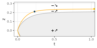
For the Exponential type
Using the normalization \(N(\lambda, \sigma) = \sigma^2 / \lambda = \sigma t\), we have:
\[\begin{align*} Z_t f_{\sigma}(z) = t \frac{\cosh \left( \frac{1-2 \lvert \lbrace z \rbrace_{-} \rvert}{t} \right)}{\sinh \left( \frac{1}{t} \right)} - t^2. \end{align*}\]We also have the following for \(t > 0\) and \(z \in [-1/2,1/2)\):
- \(\lim_{t \rightarrow +\infty} Z_t f_{\sigma}(z) = 2 z^2-2 \lvert z \rvert + 1/3\),
- \(\lim_{t \rightarrow 0} Z_t f_{\sigma}(z) = 0\),
- The smallest positive root of \(Z_t f_{\sigma}(z) = 0\) is \(z_0 = 1/2 - (t/2) \cosh^{-1}(t \sinh(1/t))\), with in particular \(z_0 \sim_{t \rightarrow 0} - t \log{t}/2\) and \(z_0 \rightarrow_{t \rightarrow +\infty} 1/2-1/(2\sqrt{3})\).
Proof (click to expand).
For \(\lambda > 0\), we consider \(x \in [-\lambda/2, \lambda/2)\), or equivalently \(z \in [-1/2, 1/2)\). The closed-form expression for the exponential type verifies:
\[\begin{align*} S_{\lambda}f_{\sigma}(x) - \frac{1}{\lambda} = \frac{1}{\sigma} \frac{\cosh \left( \frac{\lambda}{\sigma} - \frac{2\lvert x \rvert}{\sigma} \right) }{\sinh \left( \frac{\lambda}{\sigma}\right)} - \frac{1}{\lambda}. \end{align*}\]Using the normalization: \(N(\lambda, \sigma) = \frac{\sigma^2}{\lambda}\), we obtain:
\[\begin{align*} Z_t f_{\sigma}(z) =& \frac{\sigma}{\lambda} \frac{\cosh \left( \frac{\lambda}{\sigma} - \frac{2 \lambda \lvert x \rvert}{\lambda \sigma} \right) }{\sinh \left( \frac{\lambda}{\sigma}\right)} - \frac{\sigma^2}{\lambda^2} \\ =& t \frac{\cosh \left( \frac{1}{t} - \frac{2 \lvert z \rvert}{t} \right) }{\sinh \left( \frac{1}{t}\right)} - t^2 \\ =& t \frac{\cosh \left( \frac{1-2 \lvert z \rvert}{t} \right) }{\sinh \left( \frac{1}{t}\right)} - t^2. \end{align*}\]Form when \(t \rightarrow +\infty\)
With \(u:=1-2 \lvert z \rvert\), we use (the \(o\) notation is in \(+\infty\) here) that \(\cosh(u/t)=1+u^2/(2t^2)+o(1/t^2)\) and \(1/\sinh(1/t)=t-1/(6t)+o(1/t)\) so:
\[\begin{align*} \cosh(u/t)/\sinh(1/t) =& (1 + u^2/(2t^2) + o(1/t^2))(t - 1/(6t) + o(1/t)) \\ =& (t - 1/(6t) + o(1/t)) + u^2/(2t) \\ =& t + (1/6)(3u^2-1)/t + o(1/t). \end{align*}\]Hence \(Z_t f_{\sigma}(z) = (1/6)(3u^2-1) + o(1)\). Replacing \(u\) by its value, we obtain that: \(\lim_{t \rightarrow +\infty} Z_t f_{\sigma}(z) = 2 z^2-2 \lvert z \rvert + 1/3\) for \(z \in [-1/2, 1/2)\).
Form when \(t \rightarrow 0\)
The convergence to \(0\) is straightforward using the definitions of \(\sinh\) and \(\cosh\).
Roots
For \(z \in [-1/2, 1/2)\), we have \(Z_t f_{\sigma}(z) = 0\) when \(\cosh(u/t) = t \sinh(1/t)\). The final form is obtained by taking the inverse function \(\cosh^{-1}(x) = \log (x + \sqrt{x^2 -1})\) and using \(\pm z = (1-u)/2\).
We consider the smallest positive root \(z_0\) in the following (the negative is also a root, along with the translations by \(1\)).
When \(t \rightarrow 0\), we use \(\cosh(u/t) \sim \exp(u/t)\) and \(\sinh(1/t) \sim \exp(1/t)\) to get \(z_0 \sim - t \log{t}/2\).
When \(t \rightarrow +\infty\), the development is \(z_0 = 1/2-1/(2\sqrt{3}) - 1/(180 \sqrt{3} t^2) + o(1/t^2)\), giving in particular the limit \(z_0 \rightarrow_{t \rightarrow +\infty} = 1/2-1/(2\sqrt{3})\).
As before, the normalized sum \(Z_t f_{\sigma}(z)\) does not depend on \(\sigma\) (given \(t\) and \(z\)).
Restricting on the single period \(z \in [-1/2, 1/2)\), we observe in the following video:
- (left) the mapping \(z \mapsto Z_t f_{\sigma}(z)\) over time, with marked points for \(z=-1/2\) (blue), \(\pm z=1/2-1/(2\sqrt{3}) \approx 0.211\) (green), \(\pm z= 1/2-1/\sqrt{6} \approx 0.092\) (yellow) and \(z=0\) (gray); we observe a mostly increasing shape that converges to a quadratic function,
- (center) the mapping \(t \mapsto Z_t f_{\sigma}(z)\) for the \(6\) previous marked points over time; the points \(z\) have been selected to converge for large \(t\) to \(-1/6\), \(0\), \(1/6\), \(1/3\) respectively; we observe a decreasing function for the blue curve, an increasing function for the gray curve, while intermediate curves decrease before increasing,
- (right) the functions \((t, z) \mapsto \pm \left[ 1/2 - (t/2) \cosh^{-1}(t \sinh(1/t)) \right]\) represented by two gray lines and corresponding to the points were \(Z_t f_{\sigma}(z) = 0\). The inner gray region corresponds to \(Z_t f_{\sigma}(z) \geq 0\), while the outside verifies \(Z_t f_{\sigma}(z) \leq 0\). We observe as expected that the green points \(\pm z_0\) approach the frontier of the region when \(t \rightarrow +\infty\).
Additional videos of the mapping \(t \mapsto Z_t f_{\sigma}(z)\) over space, and of the unnormalized mapping \(x \mapsto S_{\lambda}f_{\sigma}(x)\) over time are provided by expanding the following tab. Other noteworthy points are also highlighted.
Additional videos (click to expand).
- Mapping \(t \mapsto Z_t f_{\sigma}(z)\) over space. Note that the colors of this video are not linked with the colors of the previous video, and the colors correspond to \(t \in \lbrace 0, 1/8, 1/4, 1 \rbrace\). We observe as before that, when \(t\) is large, \(Z_t f_{\sigma}(z) = 0\) for \(z_0=1/2-1/(2\sqrt{3}) \approx 0.21\). For this value, the function decreases until a certain \(t_0\) before increasing. Additionally, \(z_0' \approx 0.24\) seems to be the smallest positive value for which the function is always decreasing. We compute next the derivative w.r.t time to obtain those values.
- We have, for \(z \in [-1/2, 1/2)\), using \(u = 1-2 \lvert z \rvert\),
For large \(t\), \(\partial{Z_t f_{\sigma}}/\partial{t}(z) \sim (-15 u^4+30 u^2-7)/(180 t^3)\), which has a root \(u'_0 = \sqrt{1-2 \sqrt{2/15}}\) and from which we derive the point \(z'_0 := (1-u'_0)/2 = 1/2-\sqrt{1-2\sqrt{2/15}}/2 \approx 0.240\). The initial equivalence for large \(t\) was obtained by typing the following in WA:
\(\texttt{series -2*t + cosh(u/t)/sinh(1/t) + (1/t)*cosh(u/t)*cosh(1/t)/sinh(1/t)^2}\) \(\texttt{-(u/t)*sinh(u/t)/sinh(1/t) at t=+Inf}\)
For other \(t\), there does not seem to exist a closed-form expression of \(\partial{Z_t f_{\sigma}}/\partial{t}(z) = 0\) but good approximates can be obtained. For instance \(t_0 \approx 0.229\) is such that \(\partial{Z_t f_{\sigma}}/\partial{t}(z_0) = 0\)
- The following picture summarizes the previous observations. As before, the gray zone is the region where \(Z_t f_{\sigma}(z) \geq 0\), for which the function is always increasing w.r.t time. Outside, there is an intermediate region for which \(Z_t f_{\sigma}(z)\) is negative but increasing in time. Finally, the remaining region is negative and decreasing in time. Three points are marked on the figure (colors not linked with the previous figures). The gray point is located at \(t=+\infty\), \(z_0=1/2-1/(2\sqrt{3}) \approx 0.211\), for which \(Z_t f(z)=0\). The orange point is located at \(t=+\infty\), \(z'_0=1/2-\sqrt{1-2\sqrt{2/15}}/2 \approx 0.240\), for which \(Z_t f(z) = 1/3-\sqrt{2/15} \approx -0.032\) (the root of \(2z^2-2z+1/3\)). The blue point is located at \(t_0 \approx 0.2294541\), \(z=z_0\), for which \(Z_{t_0} f(z_0) \approx -0.01603669\), and \(\partial{Z_{t_0} f}/\partial{t}(z_0)=0\) by construction.
- Mapping \(x \mapsto S_{\lambda}f_{\sigma}(x)\) over time. In this unnormalized form, the \(y\)-axis is going up at a constant speed (w.r.t. \(t\)), while the \(y\)-range is shrinking. As expected, the shape is equivalent to \(z \mapsto Z_t f_{\sigma}(z)\) over time.
For the Polynomial type
Using the normalization \(N(\lambda, \sigma) = \frac{\lambda}{2} e^{2 \sigma / \lambda} = \sigma \frac{e^{2t}}{2t}\), we have:
\[\begin{align*} Z_t f_{\sigma}(z) = \frac{\cos(2 \pi z) e^{2t} - 1}{e^{2t} - 2 \cos(2 \pi z) + e^{-2t}}. \end{align*}\]We also have the following for \(t > 0\) and \(z \in [-1/2,1/2)\):
- \(\lim_{t \rightarrow +\infty} Z_t f_{\sigma}(z) = \cos(2 \pi z)\),
- \(\lim_{t \rightarrow 0} Z_t f_{\sigma}(z) = -1/2\) for \(z \neq 0\), while \(\lim_{t \rightarrow 0} Z_t f_{\sigma}(0) = +\infty\),
- The smallest positive root of \(Z_t f_{\sigma}(z) = 0\) is \(z_0 = \text{Arccos} \left( e^{-2t} \right) / (2\pi)\), with in particular \(z_0 \rightarrow_{t \rightarrow 0} 0\) and \(z_0 \rightarrow_{t \rightarrow +\infty} 1/4\).
Proof (click to expand).
For \(\lambda > 0\), we consider \(x \in [-\lambda/2, \lambda/2)\), or equivalently \(z \in [-1/2, 1/2)\). The closed-form expression for the polynomial type verifies:
\[\begin{align*} S_{\lambda}f_{\sigma}(x) - \frac{1}{\lambda} =& \frac{1}{\lambda} \frac{\sinh \left( \frac{2 \sigma}{\lambda} \right)}{\cosh \left( \frac{2 \sigma}{\lambda} \right)-\cos \left( \frac{2\pi x}{\lambda} \right)} - \frac{1}{\lambda} \\ =& \frac{1}{\lambda} \left ( \frac{\sinh (2t)}{\cosh (2t)-\cos ( 2\pi z )} - 1 \right) \\ =& \frac{1}{\lambda} \left ( \frac{e^{2t}-e^{-2t}}{e^{2t}+e^{-2t}-2\cos ( 2\pi z )} - 1 \right) \\ =& \frac{2}{\lambda} \frac{-e^{-2t}+\cos ( 2\pi z )}{e^{2t}+e^{-2t}-2\cos ( 2\pi z )} \\ =& \frac{2e^{-2t}}{\lambda} \frac{-1+\cos ( 2\pi z )e^{2t}}{e^{2t}+e^{-2t}-2\cos ( 2\pi z )}. \end{align*}\]Using the normalization: \(N(\lambda, \sigma) = \sigma e^{2t}/(2t)\), we obtain:
\[\begin{align*} Z_t f_{\sigma}(z) =& \frac{-1+\cos ( 2\pi z )e^{2t}}{e^{2t}+e^{-2t}-2\cos ( 2\pi z )}. \end{align*}\]Form when \(t \rightarrow +\infty\)
When \(t\) is large, either \(\cos(2 \pi z)=0\) and the limit is \(0\), otherwise only terms in \(e^{2t}\) are important and the limit is \(\cos(2 \pi z)\). Overall, we obtain \(\cos(2 \pi z)\) for all \(z\).
Form when \(t \rightarrow 0\)
When \(z=0\), we obtain \(Z_t f_{\sigma}(0) \sim 1/(2t)\) for small \(t\). Otherwise, \(z \neq 0\) and \(\cos(2 \pi z) \neq 1\), and we obtain \(Z_t f_{\sigma}(0) \sim -1/2\) for small \(t\).
Roots
For \(t>0\), the denominator term is always positive, so the root \(z_0\) verifies: \(\cos(2\pi z)=e^{-2t}\). We deduce that the positive root is: \(z_0 = \text{Arccos} \left( e^{-2t} \right) / (2\pi)\). We can also see that \(t = -\frac{1}{2} \log \cos ( 2 \pi z)\).
As before, the normalized sum \(Z_t f_{\sigma}(z)\) does not depend on \(\sigma\) (given \(t\) and \(z\)).
Restricting on the single period \(z \in [-1/2, 1/2)\), we observe in the following video:
- (left) the mapping \(z \mapsto Z_t f_{\sigma}(z)\) over time, with marked points for \(z=-1/2\) (blue), \(z=\pm 1/4\) (green), \(z= \pm 1/6\) (yellow) and \(z=0\) (gray); we observe an interesting flattening of the initial peak towards the cosinus function,
- (center) the mapping \(t \mapsto Z_t f_{\sigma}(z)\) for the \(6\) previous marked points over time; the points \(z\) have been selected to converge for large \(t\) to \(-1\), \(0\), \(1/2\), \(1\) respectively; we observe a decreasing function for the blue and gray curves, while intermediate yellow and green curves increase,
- (right) the functions \(t \mapsto \pm \text{Arccos} \left( e^{-2t} \right) / (2\pi)\) represented by two gray lines and corresponding to the points were \(Z_t f_{\sigma}(z) = 0\). The inner gray region corresponds to \(Z_t f_{\sigma}(z) \geq 0\), while the outside verifies \(Z_t f_{\sigma}(z) \leq 0\). We observe as expected that the green points \(\pm 1/4\) approach the frontier of the region when \(t \rightarrow +\infty\).
Additional videos of the mapping \(t \mapsto Z_t f_{\sigma}(z)\) over space, and of the unnormalized mapping \(x \mapsto S_{\lambda}f_{\sigma}(x)\) over time are provided by expanding the following tab.
Additional videos (click to expand).
- Mapping \(t \mapsto Z_t f_{\sigma}(z)\) over space. Note that the colors of this video are not linked with the colors of the previous video, and the colors correspond to \(t \in \lbrace 0, 0.35, 0.55, 2 \rbrace\) (the peak at \(z=0\) is \(2\) at \(t = \log(2)/2 \approx 0.35\), and is \(1.5\) at \(\log(3)/2 \approx 0.55\)).
- We compute next the derivative w.r.t time. We have for \(z \in [-1/2, 1/2)\), with \(A = \cos \left( 2 \pi z \right)\):
In particular, \(\partial{Z_t f_{\sigma}}/\partial{t}(z)=0\) when \(A^2-Ae^{-2t}-1/2+e^{-4t}/2 = 0\), which is quadratic in \(A\), and for which we deduce the roots of the form \(t = f(z)\).
- The following picture summarizes the information regarding \(Z_t f_{\sigma}\). As before, the gray zone is the region where \(Z_t f_{\sigma}(z) \geq 0\). The orange curves represent the positions where \(\partial{Z_t f_{\sigma}}/\partial{t}(z)=0\). Different points are marked on the figure (colors not linked with the previous figures). The gray point is located at \(t=+\infty\), \(z_0=1/4\), for which \(Z_t f(z)=0\). The bottom-right orange point is the smallest positive value \(z=1/8=0.125\) for which the function is always increasing. The top-right orange point is the smallest positive value \(z=3/8=0.375\) for which the function is always decreasing. The other orange points on the left are located at \(z=0\) and \(z=1/4\).
- Mapping \(x \mapsto S_{\lambda}f_{\sigma}(x)\) over time. In this unnormalized form, the \(y\)-axis is going up at a constant speed (w.r.t. \(t\)), while the \(y\)-range is shrinking exponentially. As expected, the shape is equivalent to \(z \mapsto Z_t f_{\sigma}(z)\) over time.
Alternative normalization \(N(\lambda, \sigma) = \frac{\sigma}{2t} \left( e^{2t} - 1\right)\) (click to expand).
This normalization allows the function to be bounded for \(t\) small (instead of being equivalent to \(1/(2t)\) in \(z=0\) for the original normalization).
- Mapping \(t \mapsto Z_t f_{\sigma}(z)\) over time, with marked points for \(z=-1/2\) (blue), \(z=\pm 1/4\) (green), \(z= \pm 1/6\) (yellow) and \(z=0\) (gray). In the middle plot, we observe a decreasing function for the blue curve, an increasing function for the gray curve, while intermediate curves decrease before increasing (this behavior is similar to the exponential case, cf. also the additional content below). In the right plot, the representation is unchanged compared to the original normalization.
- Mapping \(t \mapsto Z_t f_{\sigma}(z)\) over space. Note that the colors of this video are not linked with the colors of the previous video, and the colors correspond to \(t \in \lbrace 0, 0.26, 0.55, 2 \rbrace\) (the value at \(z=-1/2\) is \(-1/4\) at \(t = \log(5/3)/2 \approx 0.26\), and is \(-1/2\) at \(\log(3)/2 \approx 0.55\)).
- We compute next the derivative w.r.t time for this normalization. We have, for \(z \in [-1/2, 1/2)\), using \(A = \cos(2 \pi z)\)
We obtain that \(\partial{Z_t f_{\sigma}}/\partial{t}(z) = 0\) when \(z = \text{Arccos}\left( e^{-4t}/2 + e^{-2t} - 1/2 \right) / (2 \pi)\)
- The following picture summarizes the information regarding \(Z_t f_{\sigma}\), that is qualitatively similar to the one described for the Exponential type. As before, the gray zone is the region where \(Z_t f_{\sigma}(z) \geq 0\), for which the function is always increasing w.r.t time. Outside, there is an intermediate region for which \(Z_t f_{\sigma}(z)\) is negative but increasing in time. Finally, the remaining region is negative and decreasing in time. Three points are marked on the figure (colors not linked with the previous figures). The gray point is located at \(t=+\infty\), \(z_0=1/4\), for which \(Z_t f(z)=0\). The orange point is located at \(t=+\infty\), \(z'_0=1/3\), for which \(Z_t f(z'_0) = -1/2\). The blue point is located at \(t_0 = \log \left( 1 + \sqrt{2} \right) / 2 \approx 0.44\), \(z=z_0\), for which \(Z_{t_0} f(z_0) = 1/2-\sqrt{2}/2 \approx -0.21\), and \(\partial{Z_{t_0} f}/\partial{t}(z_0)=0\) by construction.
Alternative normalization \(N(\lambda, \sigma) = \frac{\sigma}{2t} \left( e^{2t} - 1 - 2t \right)\) (click to expand).
This normalization has the advantage to make \(Z_t f_{\sigma}(0)\) asymptotically equivalent to \(t\) for \(t\) small (instead of \(1/(2t)\) of the original normalization), so that the shape remains consistent with the normalizations applied in the Linear and the Exponential types.
- Mapping \(t \mapsto Z_t f_{\sigma}(z)\) over time, with marked points for \(z=-1/2\) (blue), \(z=\pm 1/4\) (green), \(z= \pm 1/6\) (yellow) and \(z=0\) (gray). In the middle plot, we observe a decreasing function for the blue curve, an increasing function for the gray curve, while intermediate curves decrease before increasing (the behavior is more complex than for the original normalization of even compared to the exponential case, cf. the additional content below). In the right plot, the representation is unchanged compared to the original normalization.
- Mapping \(t \mapsto Z_t f_{\sigma}(z)\) over space. Note that the colors of this video are not linked with the colors of the previous video, and the colors correspond to \(t \in \lbrace 0, 1/2, 1, 2 \rbrace\). We observe as before that, when \(t\) is large, \(Z_t f_{\sigma}(z) = 0\) for \(z_0=1/4\). For this value, the function decreases until a certain \(t_0\) before increasing. Additionally, \(z_0' \approx 0.28\) seems to be the smallest positive value for which the function is always decreasing.
- We compute next the derivative w.r.t time for this normalization. We have, for \(z \in [-1/2, 1/2)\), using \(A = \cos(2 \pi z)\)
For large \(t\), the root of \(\partial{Z_t f_{\sigma}}/\partial{t}(z)\) converges to \(z_0=1/4\). For the other point of interest in the behavior of the function, we rely on numerical approximations.
- The following picture summarizes the information regarding \(Z_t f_{\sigma}\). As before, the gray zone is the region where \(Z_t f_{\sigma}(z) \geq 0\), for which the function is always increasing w.r.t time. Outside, there is an intermediate region for which \(Z_t f_{\sigma}(z)\) is negative but increasing in time. The remaining region is negative and decreasing in time. Contrary to the exponential case, there is the zone \(z \in (0.25, 0.28]\) for which the function is decreasing, increasing and finally decreasing again over time. Three points are marked on the figure (colors not linked with the previous figures). The gray point is located at \(t=+\infty\), \(z_0=1/4\), for which \(Z_t f(z)=0\). The orange point is the smallest positive value \(z_0'\) for which the function is always decreasing, and \(z_0' \approx 0.2808306\). The corresponding time value is \(t_0' \approx 1.750595\), for which \(Z_{t_0'} f(z_0') \approx -0.1925\), and \(\partial{Z_{t_0'} f}/\partial{t}(z_0')=0\) by construction. The blue point is located at \(t_0 \approx 0.6835852\), \(z_0=1/4\), for which \(Z_{t_0} f(z_0) \approx -0.0949451\) and \(\partial{Z_{t_0} f}/\partial{t}(z_0)=0\) by construction.
For the Gaussian type
Using the normalization \(N(\lambda, \sigma) = \frac{\lambda}{2} e^{\pi \sigma^2 / \lambda^2} = \sigma \frac{e^{\pi t^2}}{2t}\), we have:
\[\begin{align*} Z_t f_{\sigma}(z) = \cos(2 \pi z) + \sum_{k=2}^{+\infty} e^{-\pi t^2 (k^2 -1)} \cos \left( 2 k \pi z \right). \end{align*}\]We also have the following for \(t > 0\) and \(z \in [-1/2,1/2)\):
- \(\lim_{t \rightarrow +\infty} Z_t f_{\sigma}(z) = \cos(2 \pi z)\),
- \(\lim_{t \rightarrow 0} Z_t f_{\sigma}(z) = -1/2\) for \(z \neq 0\), while \(\lim_{t \rightarrow 0} Z_t f_{\sigma}(0) = +\infty\),
- The smallest positive root of \(Z_t f_{\sigma}(z) = 0\) verifies \(z_0 \sim_{t \rightarrow 0} \sqrt{- t^2 \log(t) / \pi}\) with in particular \(z_0 \rightarrow_{t \rightarrow 0} 0\), while \(z_0 \rightarrow_{t \rightarrow +\infty} 1/4\).
Proof (click to expand).
For \(\lambda > 0\), we consider \(x \in [-\lambda/2, \lambda/2)\), or equivalently \(z \in [-1/2, 1/2)\). The closed-form expression for the Gaussian type verifies:
\[\begin{align*} S_{\lambda}f_{\sigma}(x) - \frac{1}{\lambda} =& \frac{1}{\lambda} \left( \vartheta_3 \left( \frac{\pi x}{\lambda}, e^{-\frac{\pi \sigma^2}{\lambda^2}} \right) - 1 \right) \\ =& \frac{t}{\sigma} \left( \vartheta_3 \left( \pi z, e^{-\pi t^2} \right) - 1 \right) \\ =& \frac{t}{\sigma} \left( -1 + \sum_{k=-\infty}^{+\infty} e^{-\pi k^2 t^2} e^{2ik \pi z} \right) \\ =& \frac{2t}{\sigma} \left( \sum_{k=1}^{+\infty} e^{-\pi k^2 t^2} \cos ( 2k \pi z) \right). \end{align*}\]Using the normalization: \(N(\lambda, \sigma) = \sigma e^{\pi t^2}/(2t)\), we obtain:
\[\begin{align*} Z_t f_{\sigma}(z) =& \sum_{k=1}^{+\infty} e^{\pi t^2} e^{-\pi k^2 t^2} \cos ( 2k \pi z) \\ =& \cos(2 \pi z) + \sum_{k=2}^{+\infty} e^{-\pi t^2 (k^2 -1)} \cos \left( 2 k \pi z \right). \end{align*}\]Form when \(t \rightarrow +\infty\)
When \(t\) is large, the only dominant term is the first term \(\cos(2 \pi z)\) for all \(z\).
Form when \(t \rightarrow 0\)
For \(t\) small, the formula obtained for \(Z_t f_{\sigma}\) is not convenient, and we need to apply the Poisson summation formula again, now with \(h: x \mapsto e^{-\pi x^2}\), for which \(\mathcal{F}h = h\). In details, we can apply formally the original formula:
\[\frac{1}{\lambda} \sum_{k=-\infty}^{+\infty} \mathcal{F}f \left( \frac{k}{\lambda} \right) e^{2i\pi \frac{k}{\lambda} x} = \sum_{k=-\infty}^{+\infty} f(x+k\lambda)\]by replacing arbitrary the free parameters with \(x=z/t\), \(\lambda = 1/t\), and \(f = h\), to retrieve:
\[\begin{align*} t \sum_{k=-\infty}^{+\infty} h(tk) e^{2i\pi t k z/t} =& \sum_{k=-\infty}^{+\infty} h(z/t +k/t)\\ t \sum_{k=-\infty}^{+\infty} e^{-\pi t^2 k^2} e^{2i\pi k z} =& \sum_{k=-\infty}^{+\infty} e^{-\pi (z+k)^2/t^2}\\ \vartheta_3 \left( \pi z, e^{-\pi t^2} \right) =& \frac{1}{t} \sum_{k=-\infty}^{+\infty} e^{-\pi (z+k)^2/t^2}. \end{align*}\]We then deduce:
\[\begin{align*} S_{\lambda}f_{\sigma}(x) - \frac{1}{\lambda} =& \frac{t}{\sigma} \left( \vartheta_3 \left( \pi z, e^{-\pi t^2} \right) - 1 \right) \\ =& \frac{t}{\sigma} \left( - 1 + \frac{1}{t} \sum_{k=-\infty}^{+\infty} e^{-\pi (z+k)^2/t^2} \right) \end{align*}\]and:
\[\begin{align*} Z_t f_{\sigma}(z) =& \frac{e^{\pi t^2}}{2} \left( -1 + \frac{1}{t} \sum_{k=-\infty}^{+\infty} e^{-\pi (z+k)^2/t^2} \right) \\ =& e^{\pi t^2} \left( -\frac{1}{2} + \frac{1}{2t} e^{-\pi z^2/t^2} + \frac{1}{t} \sum_{k=1}^{+\infty} e^{-\pi (z+k)^2/t^2} \right). \end{align*}\]When \(z=0\), we obtain \(Z_t f_{\sigma}(0) \sim 1/(2t)\) for small \(t\). Otherwise, \(z \neq 0\) and we obtain \(Z_t f_{\sigma}(0) \sim -1/2\) for small \(t\).
Roots
For \(t\) positive and small, we can use the formula obtained in the previous paragraph and solve the equation:
\[e^{\pi t^2} \left( -\frac{1}{2} + \frac{1}{2t} e^{-\pi z^2/t^2} \right) = 0,\]for which we obtain that the positive root verifies: \(z_0 \sim_{t \rightarrow 0} \sqrt{-t^2 \log(t) / \pi},\)
which is remarkably accurate until \(t \approx 0.5\). In particular the limit in \(t = 0\) is \(z_0 \rightarrow 0\).
For \(t\) large, we use the initial formula that shows that the dominant term is \(\cos(2 \pi z)\) for all \(z\), for which we deduce that the limit in \(t = +\infty\) is \(z_0 \rightarrow 1/4\).
As before, the normalized sum \(Z_t f_{\sigma}(z)\) does not depend on \(\sigma\) (given \(t\) and \(z\)).
Restricting on the single period \(z \in [-1/2, 1/2)\), we observe in the following video:
- (left) the mapping \(z \mapsto Z_t f_{\sigma}(z)\) over time, with marked points for \(z=-1/2\) (blue), \(z=\pm 1/4\) (green), \(z= \pm 1/6\) (yellow) and \(z=0\) (gray); we observe a sharp flattening of the initial peak towards the cosinus function,
- (center) the mapping \(t \mapsto Z_t f_{\sigma}(z)\) for the \(6\) previous marked points over time; the points \(z\) have been selected to converge for large \(t\) to \(-1\), \(0\), \(1/2\), \(1\) respectively; we observe a decreasing function for the blue and gray curves, while the other yellow and green curves seem to decrease before increasing,
- (right) the functions represented by two gray lines and corresponding to the points were \(Z_t f_{\sigma}(z) = 0\). The inner gray region corresponds to \(Z_t f_{\sigma}(z) \geq 0\), while the outside verifies \(Z_t f_{\sigma}(z) \leq 0\). We observe as expected that the green points \(\pm 1/4\) approach the frontier of the region when \(t \rightarrow +\infty\).
Additional videos of the mapping \(t \mapsto Z_t f_{\sigma}(z)\) over space, and of the unnormalized mapping \(x \mapsto S_{\lambda}f_{\sigma}(x)\) over time are provided by expanding the following tab.
Additional videos (click to expand).
- Mapping \(t \mapsto Z_t f_{\sigma}(z)\) over space. Note that the colors of this video are not linked with the colors of the previous video, and the colors correspond to \(t \in \lbrace 0, 1/4, 1/3, 1 \rbrace\).
-
We rely on numerical approximations for solving \(\partial{Z_t f_{\sigma}}/\partial{t}(z)=0\).
-
The following picture summarizes the information regarding \(Z_t f_{\sigma}\). As before, the gray zone is the region where \(Z_t f_{\sigma}(z) \geq 0\). The orange curves represent the positions where \(\partial{Z_t f_{\sigma}}/\partial{t}(z)=0\). Different points are marked on the figure (colors not linked with the previous figures). Since the behavior for large \(t\) is similar to the polynomial case, the marked points on the right part of the figure are identical: the gray point is located at \(t=+\infty\), \(z_0=1/4\), for which \(Z_t f(z)=0\); the bottom-right orange point is the smallest positive value \(z=1/8=0.125\) for which the function is always increasing; and the top-right orange point is the smallest positive value \(z=3/8=0.375\) for which the function is always decreasing. The remaining orange point on the left is located at \(z=0\).

- Mapping \(x \mapsto S_{\lambda}f_{\sigma}(x)\) over time. In this unnormalized form, the \(y\)-axis is going up at a constant speed (w.r.t. \(t\)), while the \(y\)-range is shrinking exponentially. As expected, the shape is equivalent to \(z \mapsto Z_t f_{\sigma}(z)\) over time.
Alternative normalization \(N(\lambda, \sigma) = \frac{\sigma}{2t} \left( e^{\pi t^2} - 1 \right)\) (click to expand).
This normalization allows the function to have a flat shape for small \(t\), as for the normalizations applied in the Linear and the Exponential types.
- Mapping \(t \mapsto Z_t f_{\sigma}(z)\) over time, with marked points for \(z=-1/2\) (blue), \(z=\pm 1/4\) (green), \(z= \pm 1/6\) (yellow) and \(z=0\) (gray). In the middle plot, we observe a decreasing function for the blue curve, an increasing function for the gray curve, while intermediate curves decrease before increasing (the behavior is more complex than for the exponential and the polynomial cases, cf. the additional content below). In the right plot, the representation is unchanged compared to the original normalization.
- Mapping \(t \mapsto Z_t f_{\sigma}(z)\) over space. Note that the colors of this video are not linked with the colors of the previous video, and the colors correspond to \(t \in \lbrace 0, 1/4, 1/2, 1 \rbrace\).
-
As for the initial normalization, we rely on numerical approximations for solving \(\partial{Z_t f_{\sigma}}/\partial{t}(z) = 0\).
-
The following picture summarizes the information regarding \(Z_t f_{\sigma}\). As before, the gray zone is the region where \(Z_t f_{\sigma}(z) \geq 0\), for which the function is always increasing w.r.t time. Outside, there is an intermediate region for which \(Z_t f_{\sigma}(z)\) is negative but increasing in time. The remaining region is negative and decreasing in time. The two orange points are \((0,0)\) and \((+\infty,1/4)\).
For the Sinc type
Using the normalization \(N(\lambda, \sigma) = \sigma\), we have:
\[\begin{align*} Z_t f_{\sigma}(z) =& 2 t \sum_{k=1}^{\lfloor \frac{1}{2t} \rfloor} \cos \left( 2 k \pi z \right). \end{align*}\]We also have the following for \(t > 0\) and \(z \in [-1/2,1/2)\):
- \(\lim_{t \rightarrow +\infty} Z_t f_{\sigma}(z) = 0\),
- \(\lim_{t \rightarrow 0} Z_t f_{\sigma}(z) = 0\) for \(z \neq 0\), while \(\lim_{t \rightarrow 0} Z_t f_{\sigma}(0) = 1\).
Proof (click to expand).
For \(\lambda > 0\), we consider \(x \in [-\lambda/2, \lambda/2)\), or equivalently \(z \in [-1/2, 1/2)\). The closed-form expression for the Sinc type verifies, from the previous proof:
\[\begin{align*} S_{\lambda}f_{\sigma}(x) - \frac{1}{\lambda} =& \frac{2}{\lambda} \sum_{k=1}^{\lfloor \frac{\lambda}{2\sigma} \rfloor} \cos \left( 2 \pi k x / \lambda \right) \\ =& \frac{1}{\sigma} 2 t \sum_{k=1}^{\lfloor \frac{1}{2t} \rfloor} \cos \left( 2 k \pi z \right). \end{align*}\]Using the normalization: \(N(\lambda, \sigma) = \sigma\), we obtain:
\[\begin{align*} Z_t f_{\sigma}(z) =& 2 t \sum_{k=1}^{\lfloor \frac{1}{2t} \rfloor} \cos \left( 2 k \pi z \right). \end{align*}\]As before, the normalized sum \(Z_t f_{\sigma}(z)\) does not depend on \(\sigma\) (given \(t\) and \(z\)).
Restricting on the single period \(z \in [-1/2, 1/2)\), we observe in the following video:
- (left) the mapping \(z \mapsto Z_t f_{\sigma}(z)\) over time, with marked points for \(z=-1/2\) (blue), \(z=\pm 1/4\) (green), \(z= \pm 1/6\) (yellow) and \(z=0\) (gray); we observe the cosinus function for \(t=1/2\) and the null function for larger values of \(t\).
- (center) the mapping \(t \mapsto Z_t f_{\sigma}(z)\) for the \(6\) previous marked points over time,
- (right) the gray borders correspond to the points were \(Z_t f_{\sigma}(z) = 0\). The inner gray region corresponds to \(Z_t f_{\sigma}(z) \geq 0\), while the outside verifies \(Z_t f_{\sigma}(z) \leq 0\). The zone on the right is when the function is null.
Additional videos of the mapping \(t \mapsto Z_t f_{\sigma}(z)\) over space, and of the unnormalized mapping \(x \mapsto S_{\lambda}f_{\sigma}(x)\) over time are provided by expanding the following tab.
Additional videos (click to expand).
- Mapping \(t \mapsto Z_t f_{\sigma}(z)\) over space. Note that the colors of this video are not linked with the colors of the previous video, and the colors correspond to \(t \in \lbrace 0, 1/4, 1/2, 1 \rbrace\).
- Mapping \(x \mapsto S_{\lambda}f_{\sigma}(x)\) over time.
For the Sincsquare type
Using the normalization \(N(\lambda, \sigma) = \sigma\), we have:
\[\begin{align*} Z_t f_{\sigma}(z) =& 2 t \sum_{k=1}^{\lfloor \frac{1}{t} \rfloor} \left( 1 - kt \right) \cos \left( 2 k \pi z \right). \end{align*}\]We also have the following for \(t > 0\) and \(z \in [-1/2,1/2)\):
- \(\lim_{t \rightarrow +\infty} Z_t f_{\sigma}(z) = 0\),
- \(\lim_{t \rightarrow 0} Z_t f_{\sigma}(z) = 0\) for \(z \neq 0\), while \(\lim_{t \rightarrow 0} Z_t f_{\sigma}(0) = 1\).
Proof (click to expand).
For \(\lambda > 0\), we consider \(x \in [-\lambda/2, \lambda/2)\), or equivalently \(z \in [-1/2, 1/2)\). The closed-form expression for the Sincsquare type verifies, from the previous proof:
\[\begin{align*} S_{\lambda}f_{\sigma}(x) - \frac{1}{\lambda} =& \frac{2}{\lambda} \sum_{k=1}^{\left\lfloor\frac{\lambda}{\sigma}\right\rfloor} \left( 1 - \frac{k \sigma}{\lambda} \right) \cos \left( 2\pi \frac{k}{\lambda} x \right) \\ =& \frac{2t}{\sigma} \sum_{k=1}^{\left\lfloor\frac{1}{t}\right\rfloor} \left( 1 - kt \right) \cos \left( 2 k \pi z \right). \end{align*}\]Using the normalization: \(N(\lambda, \sigma) = \sigma\), we obtain the result.
As before, the normalized sum \(Z_t f_{\sigma}(z)\) does not depend on \(\sigma\) (given \(t\) and \(z\)).
Restricting on the single period \(z \in [-1/2, 1/2)\), we observe in the following video:
- (left) the mapping \(z \mapsto Z_t f_{\sigma}(z)\) over time, with marked points for \(z=-1/2\) (blue), \(z=\pm 1/4\) (green), \(z= \pm 1/6\) (yellow) and \(z=0\) (gray); we observe (half of) the cosinus function for \(t=1/2\) that is flattened until \(t=1\); from \(t=1\), the function is null.
- (center) the mapping \(t \mapsto Z_t f_{\sigma}(z)\) for the \(6\) previous marked points over time; the sudden changes occur when the upper bound of the sum is changing, i.e. in \(1\), \(1/2\), \(1/3\), \(1/4\), etc.,
- (right) the gray borders correspond to the points were \(Z_t f_{\sigma}(z) = 0\). The inner gray region corresponds to \(Z_t f_{\sigma}(z) \geq 0\), while the outside verifies \(Z_t f_{\sigma}(z) \leq 0\). The zone from \(t=1\) (not shown) is null. Compared to Sinc, the positive regions are in a single central region, but additional interesting lobes appear for small \(t\).
Additional videos of the mapping \(t \mapsto Z_t f_{\sigma}(z)\) over space, and of the unnormalized mapping \(x \mapsto S_{\lambda}f_{\sigma}(x)\) over time are provided by expanding the following tab.
Additional videos (click to expand).
- Mapping \(t \mapsto Z_t f_{\sigma}(z)\) over space. Note that the colors of this video are not linked with the colors of the previous video, and the colors correspond to \(t \in \lbrace 0, 1/4, 1/2, 1 \rbrace\).
- Mapping \(x \mapsto S_{\lambda}f_{\sigma}(x)\) over time.
Inner lobes position.
This paragraph refers to the right plot of the Sincsquare video, showing the positive zones. The border between negative and positive zones contain inner thin lobes for small values of \(t\), that we describe in this paragraph.
By monotony argument in the shape of \(Z_t f_{\sigma}\), the cusps can only occur for \(t=1/N\) with \(N\) integer.
Then, for \(N\) integer, the function can be simplified using Fejér kernel identity:
\[\begin{align*} Z_t f_{\sigma}(z) =& 2 t \sum_{k=1}^{N} \left( 1 - k/N \right) \cos \left( 2 k \pi z \right) \\ =& 2 t \sum_{k=1}^{N-1} \left( 1 - k/N \right) \cos \left( 2 k \pi z \right) \\ =& 2 t \frac{1}{2} \left[ \frac{\sin^2 \left( N \pi z \right)}{N \sin^{2} \left( \pi z \right)} - 1 \right]. \end{align*}\]To find the position of the cusp, we solve \(Z_t f_{\sigma}(z)=0\) for those integer values, i.e. \(\sin^2(N \pi z) = N \sin^2 (\pi z)\).
Numerically, we find that \(N=21\) is the first cusp (in yellow at position \(t_0 = 0.04762\), \(z_0 = 0.06937\)), which is also the highest \(z\) position of the first inner lobe. The highest \(t\) position of the first inner lobe can be found numerically (in blue at position \(t_0 = 0.04779\), \(z_0 = 0.06838\)): in that case, \(t\) has not the form \(1/N\) and the formula does not simplify.
The cusp of the following smaller lobes (in gray) occur for \(N=61, 120, 199\).
Area of the parametric curve \((S_\lambda f_\sigma, S_\lambda g_\sigma)\)
The following paragraphs are written with the help of Claude Opus 4.6.
The parametric curve \((S_\lambda f_\sigma(x), S_\lambda g_\sigma(x))\) for \(x \in [-\lambda/2, \lambda/2)\) encloses an area given by Green’s theorem:
\[\mathcal{A} = \frac{1}{2}\left|\int_{-\lambda/2}^{\lambda/2}\left(S_\lambda f_\sigma \frac{d(S_\lambda g_\sigma)}{dx} - S_\lambda g_\sigma \frac{d(S_\lambda f_\sigma)}{dx}\right)dx\right|.\]This area is (provided that the right-term sum converges, which holds for all types except Rectangular):
\[\mathcal{A} = \frac{8\pi^2}{\lambda^3}\sum_{k=1}^{\infty} k^2\left[\mathcal{F}f_\sigma\left(\frac{k}{\lambda}\right)\right]^2.\]Proof (click to expand).
We write \(X(x) = S_\lambda f_\sigma(x) = \frac{1}{\lambda} + \widetilde{X}(x)\) where:
\[\widetilde{X}(x) = \frac{2}{\lambda}\sum_{j=1}^{\infty} \mathcal{F}f_\sigma\left(\frac{j}{\lambda}\right) \cos\left(2\pi \frac{j}{\lambda}x\right),\] \[Y(x) = S_\lambda g_\sigma(x) = -\frac{4\pi}{\lambda^2}\sum_{j=1}^{\infty} j\,\mathcal{F}f_\sigma\left(\frac{j}{\lambda}\right) \sin\left(2\pi \frac{j}{\lambda}x\right).\]Since \(\frac{1}{\lambda}\) is constant, \(\frac{dX}{dx} = \frac{d\widetilde{X}}{dx}\), and:
\[X \frac{dY}{dx} - Y \frac{dX}{dx} = \frac{1}{\lambda}\frac{dY}{dx} + \widetilde{X}\frac{dY}{dx} - Y\frac{d\widetilde{X}}{dx}.\]The first term integrates to zero over a full period by periodicity: \(\int_{-\lambda/2}^{\lambda/2}\frac{dY}{dx}\,dx = Y(\lambda/2) - Y(-\lambda/2) = 0\).
The derivatives with respect to \(x\) are:
\[\frac{d\widetilde{X}}{dx} = -\frac{4\pi}{\lambda^2}\sum_{k=1}^{\infty} k\,\mathcal{F}f_\sigma\left(\frac{k}{\lambda}\right)\sin\left(2\pi\frac{k}{\lambda}x\right),\] \[\frac{dY}{dx} = -\frac{8\pi^2}{\lambda^3}\sum_{k=1}^{\infty} k^2\,\mathcal{F}f_\sigma\left(\frac{k}{\lambda}\right)\cos\left(2\pi\frac{k}{\lambda}x\right).\]Writing \(a_k := \mathcal{F}f_\sigma(k/\lambda)\) for brevity, the two products are:
\[\widetilde{X}\frac{dY}{dx} = -\frac{16\pi^2}{\lambda^4}\sum_{j,k=1}^{\infty} k^2\,a_j\,a_k\,\cos\left(2\pi\frac{j}{\lambda}x\right)\cos\left(2\pi\frac{k}{\lambda}x\right),\] \[Y\frac{d\widetilde{X}}{dx} = \frac{16\pi^2}{\lambda^4}\sum_{j,k=1}^{\infty} jk\,a_j\,a_k\,\sin\left(2\pi\frac{j}{\lambda}x\right)\sin\left(2\pi\frac{k}{\lambda}x\right).\]Combining:
\[\widetilde{X}\frac{dY}{dx} - Y\frac{d\widetilde{X}}{dx} = -\frac{16\pi^2}{\lambda^4}\sum_{j,k=1}^{\infty} a_j\,a_k\left[k^2\cos\left(2\pi\frac{j}{\lambda}x\right)\cos\left(2\pi\frac{k}{\lambda}x\right) + jk\sin\left(2\pi\frac{j}{\lambda}x\right)\sin\left(2\pi\frac{k}{\lambda}x\right)\right].\]Integrating over \([-\lambda/2, \lambda/2)\) using the orthogonality relations:
\[\int_{-\lambda/2}^{\lambda/2}\cos\left(2\pi\frac{j}{\lambda}x\right)\cos\left(2\pi\frac{k}{\lambda}x\right)dx = \frac{\lambda}{2}\,\delta_{jk}, \qquad \int_{-\lambda/2}^{\lambda/2}\sin\left(2\pi\frac{j}{\lambda}x\right)\sin\left(2\pi\frac{k}{\lambda}x\right)dx = \frac{\lambda}{2}\,\delta_{jk},\]all cross terms (\(j \neq k\)) vanish. For \(j = k\), the cosine integral contributes \(k^2 a_k^2 \cdot \lambda/2\) and the sine integral contributes \(k^2 a_k^2 \cdot \lambda/2\), giving:
\[\int_{-\lambda/2}^{\lambda/2}\left(\widetilde{X}\frac{dY}{dx} - Y\frac{d\widetilde{X}}{dx}\right)dx = -\frac{16\pi^2}{\lambda^4} \cdot 2 \cdot \frac{\lambda}{2} \sum_{k=1}^{\infty} k^2\,a_k^2 = -\frac{16\pi^2}{\lambda^3}\sum_{k=1}^{\infty} k^2\,a_k^2.\]Therefore the area (unsigned and without further normalization) is:
\[\mathcal{A} = \frac{8\pi^2}{\lambda^3}\sum_{k=1}^{\infty} k^2\left[\mathcal{F}f_\sigma\left(\frac{k}{\lambda}\right)\right]^2.\]The following table shows the closed-form expression of \(\sigma^3 \mathcal{A}\) and its behavior for \(t \to \infty\), with \(t := \sigma/\lambda\).
| $$\text{Type}$$ | $$\sigma^3 \mathcal{A}$$ | $$\sigma^3 \mathcal{A}$$ for $$t \to \infty$$ | $$\text{video}$$ |
| Rectangular | $$0$$ (degenerate) | $$0$$ | |
| Linear | $$\displaystyle \frac{2 \min\left(\lbrace t \rbrace, 1-\lbrace t \rbrace\right)}{t}$$ | oscillates in $$\displaystyle \left[0, \frac{1}{t}\right]$$ | |
| Exponential | $$\displaystyle 2\left(\coth \frac{1}{t} - \frac{1}{t \sinh^2 \frac{1}{t}}\right)$$ | $$\displaystyle \sim \frac{4}{3t}$$ | |
| Polynomial | $$\displaystyle \frac{2\pi^2 t^3 \cosh(2t)}{\sinh^3(2t)}$$ | $$\sim 8\pi^2 t^3 e^{-4t}$$ | |
| Gaussian | $$\displaystyle 8\pi^2 t^3 \sum_{k=1}^{\infty} k^2 e^{-2\pi k^2 t^2}$$ | $$\sim 8\pi^2 t^3 e^{-2\pi t^2}$$ | |
| Sinc | $$\displaystyle \frac{4\pi^2 t^3 N(N+1)(2N+1)}{3}$$, $$N := \left\lfloor \frac{1}{2t} \right\rfloor$$ | $$= 0$$ for $$t > 1/2$$ | |
| Sincsquare | $$\displaystyle 8\pi^2 t^3 \sum_{k=1}^{\left\lfloor 1/t \right\rfloor} k^2 \left(1-kt\right)^2$$ | $$= 0$$ for $$t \geq 1$$ |
Proof (click to expand).
Rectangular. Since \(S_{\lambda}g_{\sigma}(x) = 0\) for all regular \(x\), the parametric curve is degenerate (it traces a segment on the horizontal axis), so \(\mathcal{A} = 0\). The Fourier sum \(\sum k^2 \text{sinc}^2(kt) = \frac{1}{\pi^2 t^2} \sum \sin^2(\pi k t)\) diverges, so the Fourier area formula does not apply to this type.
Linear. Using \(k^2 \text{sinc}^4(kt) = \frac{\sin^4(\pi k t)}{\pi^4 t^4 k^2}\) and the decomposition \(\sin^4(\pi k t) = \frac{3}{8} - \frac{1}{2}\cos(2\pi k t) + \frac{1}{8}\cos(4\pi k t)\), together with the identity \(\sum_{k=1}^{\infty} \frac{\cos(2\pi k \alpha)}{k^2} = \pi^2 B_2(\lbrace \alpha \rbrace)\) where \(B_2(x) = x^2-x+\frac{1}{6}\), we obtain:
\[\sigma^3 \mathcal{A} = \frac{1}{t}\left[\frac{1}{2} - 4 B_2(\lbrace t \rbrace) + B_2(\lbrace 2t \rbrace)\right].\]For \(\lbrace t \rbrace \in [0, \frac{1}{2})\): \(\lbrace 2t \rbrace = 2\lbrace t \rbrace\), and the bracket simplifies to \(\frac{1}{2} - 4(\lbrace t \rbrace^2 - \lbrace t \rbrace + \frac{1}{6}) + (4\lbrace t \rbrace^2 - 2\lbrace t \rbrace + \frac{1}{6}) = 2\lbrace t \rbrace\).
For \(\lbrace t \rbrace \in [\frac{1}{2}, 1)\): \(\lbrace 2t \rbrace = 2\lbrace t \rbrace - 1\), and the bracket simplifies to \(2(1-\lbrace t \rbrace)\).
In both cases: \(\sigma^3 \mathcal{A} = \frac{2\min(\lbrace t \rbrace, 1-\lbrace t \rbrace)}{t}\), which is the tent function divided by \(t\), \(1\)-periodic, vanishing at integers and peaking at \(1/t\) at half-integers.
Exponential. From the identity \(\sum_{k=1}^{\infty} \frac{k^2}{(1+b^2 k^2)^2} = \frac{\pi}{4b^4}\left(\frac{b}{\tanh(\pi/b)} - \frac{\pi}{\sinh^2(\pi/b)}\right)\) with \(b = \pi t\), we derive after simplification:
\[\sigma^3 \mathcal{A} = 2\left(\coth \frac{1}{t} - \frac{1}{t \sinh^2 \frac{1}{t}}\right).\]The series expansion \(\coth u - u\,\text{cosech}^2 u = \frac{2u}{3} - \frac{4u^3}{45} + \cdots\) with \(u = 1/t\) gives \(\sigma^3 \mathcal{A} \sim \frac{4}{3t}\) for \(t\) large.
Polynomial. Using \(\mathcal{F}f_\sigma(k/\lambda) = e^{-2kt}\) and the generating function \(\sum_{k=1}^{\infty} k^2 q^k = q(1+q)/(1-q)^3\) with \(q = e^{-4t}\):
\[\sum_{k=1}^{\infty} k^2 e^{-4kt} = \frac{e^{-4t}(1+e^{-4t})}{(1-e^{-4t})^3} = \frac{\cosh(2t)}{4\sinh^3(2t)},\]so \(\sigma^3 \mathcal{A} = \frac{2\pi^2 t^3 \cosh(2t)}{\sinh^3(2t)}\). For \(t\) large: \(\cosh(v)/\sinh^3(v) \sim 4 e^{-2v}\), giving \(\sigma^3 \mathcal{A} \sim 8\pi^2 t^3 e^{-4t}\).
Gaussian. Using \(\mathcal{F}f_\sigma(k/\lambda) = e^{-\pi k^2 t^2}\), the sum \(\sum k^2 e^{-2\pi k^2 t^2}\) is related to the second derivative of the Jacobi theta function: \(\sigma^3 \mathcal{A} = -\pi^2 t^3 \vartheta_3''(0, e^{-2\pi t^2})\). For \(t\) large, the dominant \(k=1\) term gives \(\sigma^3 \mathcal{A} \sim 8\pi^2 t^3 e^{-2\pi t^2}\).
Sinc. From \(\mathcal{F}f_\sigma(k/\lambda) = \mathbf{1}_{k \leq 1/(2t)}\), only \(N = \lfloor 1/(2t) \rfloor\) terms contribute, giving \(\sigma^3 \mathcal{A} = \frac{4\pi^2 t^3 N(N+1)(2N+1)}{3}\). For \(t > 1/2\): \(N = 0\) and \(\mathcal{A} = 0\). The area jumps discontinuously at each \(t = 1/(2n)\), with jump magnitude \(\pi^2/n\).
Sincsquare. From \(\mathcal{F}f_\sigma(k/\lambda) = (1-kt)\mathbf{1}_{k \leq 1/t}\): only \(N = \lfloor 1/t \rfloor\) terms contribute. For \(t \geq 1\): \(N = 0\) and \(\mathcal{A} = 0\) exactly. The onset is continuous: for \(t \lesssim 1\), only \(k=1\) contributes, giving \(\sigma^3 \mathcal{A} \sim 8\pi^2(1-t)^2/t\).
We describe all the curves above (area of the parametric curve \((Sf, Sg)\) without any normalization) for the setting \(\sigma=1\). For \(\sigma \neq 1\), the \(x\)-axis part scales in \(\sigma\) and the \(y\)-axis part scales in \(\sigma^2\), explaining the \(\sigma^3\) term in the area. The videos keep an aspect ratio of 1.
-
For the Linear type, the parametric curve is a rectangle that drifts rightward over time. From \(t=0\) to \(t=0.5\), it is a fixed rectangle \([0,1] \times [-1,1]\). Then it shrinks from the left (the peak stays at \(1\)) until \(t=1\), where it collapses to a vertical segment. It then re-expands and resumes drifting, with maximum width at half-integers \(t = 1/2, 3/2, 5/2, \ldots\) and zero width at integers \(t = 1, 2, 3, \ldots\) The maximum width decays as \(1/(2t)\), so the oscillations become smaller and smaller.
-
For the Exponential type, the parametric curve starts as a triangle with vertex at \((0,0)\) and base segment \(\lbrace 1 \rbrace \times [-1/2, 1/2]\). From around \(t \approx 0.3\), the vertex squishes into a rounded cusp, with the profile progressively shaping into a parabola. From around \(t \approx 0.5\), the base segment begins drifting rightward (at position \(\coth(1/t) \approx 1.04\) at \(t=0.5\) as \(t\) is small, then approximately \(t\) for larger values). The parabola gets closer to the segment, and the area decays as \(4/(3t)\). Unlike the Linear type, there are no oscillations, the width decreases monotonically.
-
For the Polynomial type, the parametric curve is a smooth closed loop. For small \(t\), the curve shows a vertical spike peaking at \((0,0)\) and a rounder cap with height \([-2,2]\) near \((1,0)\). From around \(t \approx 0.5\), the curve smooths into an ellipse shape that is then shrinking. Regarding width, the left side initially moves towards the right side, then both sides drift rightward while the width reduces, and both converge towards \(t\). The height starts at \([-2,2]\), crosses \([-1,1]\) around \(t=1.9\) and keeps shrinking. Both width and height decay exponentially.
-
For the Gaussian type, the curve is similar to the Polynomial type but with much faster shrinking. Initially, the curve has height \([-\sqrt{2\pi/e}, \sqrt{2\pi/e}] \approx [-1.52, 1.52]\) and width \([0,1]\). Unlike the Polynomial case, there is almost no visible spike at \((0,0)\). The shrinking starts around \(t = 0.5\) and is super-exponential. By \(t = 1.5\), the curve is essentially a point drifting at position \(t\).
-
For the Sinc type, for \(t>1/2\), the curve collapses to a single point. For \(1/4 < t \leq 1/2\), the curve is a single smooth ellipse. For smaller \(t\), the curve self-intersects and traces multiple oscillating loops. The area given by Green’s theorem is the algebraic (signed) area of these overlapping loops, not the area of a single enclosed region.
-
For the Sincsquare type, for \(t \geq 1\), the curve is a single point. For \(1/2 \leq t < 1\), the curve is a single smooth ellipse. For smaller \(t\), the main ellipse is accompanied by small petal-like loops near the origin that grow in number as \(t\) decreases. Unlike the Sinc type, \(S_\lambda f\) stays non-negative. The area is again algebraic (signed over the overlapping loops).
Normalized area of the parametric curve
Setting \(\theta := 2\pi z = 2\pi x/\lambda \in [-\pi, \pi)\), the parametric curve \(\left(Z_t f_\sigma(\theta),\; \frac{d}{d\theta} Z_t f_\sigma(\theta)\right)\) for \(\theta \in [-\pi, \pi)\) encloses an area (provided that the right-term sum converges, which holds for all types except Rectangular):
\[\mathcal{A}_N = \frac{N(\lambda,\sigma)^2\, \lambda}{2\pi}\, \mathcal{A} = \pi \sum_{k=1}^{\infty} k^2\, r_k^2,\]where \(r_k := \frac{2\, N(\lambda,\sigma)}{\lambda}\, \mathcal{F}f_\sigma(k/\lambda)\) are the Fourier cosine coefficients of \(Z_t f_\sigma\) in \(\theta\), and \(N(\lambda,\sigma)\) is a normalization that changes from type to type defined before.
The following table shows the closed-form expression of \(\mathcal{A}_N\) and its behavior for \(t \to \infty\), with \(t := \sigma/\lambda\).
| $$\text{Type}$$ | $$\mathcal{A}_N$$ | $$\mathcal{A}_N$$ for $$t \to \infty$$ | $$\text{video}$$ |
| Rectangular | $$0$$ (degenerate) | $$0$$ | |
| Linear | $$\displaystyle \frac{\min\left(\lbrace t \rbrace,\, 1{-}\lbrace t \rbrace\right)}{\pi}$$ | oscillates in $$\displaystyle\left[0, \frac{1}{2\pi}\right]$$ | |
| Exponential | $$\displaystyle \frac{t}{\pi}\left(\coth \frac{1}{t} - \frac{1}{t\,\sinh^2 \frac{1}{t}}\right)$$ | $$\displaystyle \frac{2}{3\pi}$$ | |
| Polynomial | $$\displaystyle \frac{\pi\, e^{4t}\cosh(2t)}{4\,\sinh^3(2t)}$$ | $$\pi$$ | |
| Gaussian | $$\displaystyle \pi\, e^{2\pi t^2}\sum_{k=1}^{\infty} k^2\, e^{-2\pi k^2 t^2}$$ | $$\pi$$ | |
| Sinc | $$\displaystyle \frac{2\pi t^2\, N(N{+}1)(2N{+}1)}{3}$$, $$N := \left\lfloor \frac{1}{2t} \right\rfloor$$ | $$0$$ for $$t > 1/2$$ | |
| Sincsquare | $$\displaystyle 4\pi t^2 \sum_{k=1}^{\left\lfloor 1/t \right\rfloor} k^2 (1{-}kt)^2$$ | $$0$$ for $$t \geq 1$$ |
Proof (click to expand).
Derivation of the general formula
We write \(U(\theta) := Z_t f_\sigma(\theta) = \sum_{k=1}^{\infty} r_k \cos(k\theta)\) and \(W(\theta) := \frac{d}{d\theta} Z_t f_\sigma(\theta) = -\sum_{k=1}^{\infty} k\, r_k \sin(k\theta)\). The enclosed area is:
\[\mathcal{A}_N = \frac{1}{2}\left|\int_{-\pi}^{\pi}\left(U \frac{dW}{d\theta} - W \frac{dU}{d\theta}\right)d\theta\right|.\]The derivatives are \(\frac{dU}{d\theta} = -\sum_k k\,r_k \sin(k\theta)\) and \(\frac{dW}{d\theta} = -\sum_k k^2\,r_k \cos(k\theta)\). Expanding the products and integrating over \([-\pi, \pi)\) using the orthogonality relations \(\int_{-\pi}^{\pi} \cos(j\theta)\cos(k\theta)\,d\theta = \int_{-\pi}^{\pi} \sin(j\theta)\sin(k\theta)\,d\theta = \pi\delta_{jk}\), all cross terms vanish. The diagonal terms give:
\[\int_{-\pi}^{\pi} U\frac{dW}{d\theta}\,d\theta = -\pi \sum_{k=1}^{\infty} k^2\,r_k^2, \qquad \int_{-\pi}^{\pi} W\frac{dU}{d\theta}\,d\theta = -\pi \sum_{k=1}^{\infty} k^2\,r_k^2.\]Therefore:
\[\mathcal{A}_N = \frac{1}{2}\left|-2\pi\sum_{k=1}^{\infty} k^2\,r_k^2\right| = \pi\sum_{k=1}^{\infty} k^2\,r_k^2.\]The relationship with the unnormalized area follows from \(r_k = \frac{2\,N(\lambda,\sigma)}{\lambda}\,\mathcal{F}f_\sigma(k/\lambda)\), so that:
\[\mathcal{A}_N = \pi \cdot \frac{4 N^2}{\lambda^2} \sum_{k=1}^{\infty} k^2 \left[\mathcal{F}f_\sigma(k/\lambda)\right]^2 = \frac{N^2 \lambda}{2\pi} \mathcal{A}.\]Per-type computations
In each case, we use \(\mathcal{A}_N = \frac{N^2}{2\pi \sigma^2 t} \cdot (\sigma^3 \mathcal{A})\) with the values of \(N(\lambda,\sigma)\) and \(\sigma^3 \mathcal{A}\) from the previous tables.
Rectangular. \(\sigma^3 \mathcal{A} = 0\), so \(\mathcal{A}_N = 0\).
Linear. \(N = \sigma t\), so \(\frac{N^2}{2\pi \sigma^2 t} = \frac{t}{2\pi}\). Then \(\mathcal{A}_N = \frac{t}{2\pi} \cdot \frac{2\min(\lbrace t \rbrace, 1-\lbrace t \rbrace)}{t} = \frac{\min(\lbrace t \rbrace, 1-\lbrace t \rbrace)}{\pi}\). For \(t \to \infty\): oscillates in \([0, 1/(2\pi)]\).
Exponential. \(N = \sigma t\), so \(\frac{N^2}{2\pi \sigma^2 t} = \frac{t}{2\pi}\). Then \(\mathcal{A}_N = \frac{t}{2\pi} \cdot 2\left(\coth \frac{1}{t} - \frac{1}{t \sinh^2 \frac{1}{t}}\right) = \frac{t}{\pi}\left(\coth \frac{1}{t} - \frac{1}{t \sinh^2 \frac{1}{t}}\right)\). For \(t \to \infty\): using \(\coth(u) - 1/(u \sinh^2 u) \approx 2u/3\) with \(u = 1/t\), we obtain \(\mathcal{A}_N \to 2/(3\pi)\).
Polynomial. \(N = \frac{\sigma e^{2t}}{2t}\), so \(\frac{N^2}{2\pi \sigma^2 t} = \frac{e^{4t}}{8\pi t^3}\). Then \(\mathcal{A}_N = \frac{e^{4t}}{8\pi t^3} \cdot \frac{2\pi^2 t^3 \cosh(2t)}{\sinh^3(2t)} = \frac{\pi e^{4t} \cosh(2t)}{4 \sinh^3(2t)}\). For \(t \to \infty\): \(e^{4t} \cosh(2t) / \sinh^3(2t) \to e^{4t} \cdot (e^{2t}/2) / (e^{6t}/8) = 4\), so \(\mathcal{A}_N \to \pi\).
Gaussian. \(N = \frac{\sigma e^{\pi t^2}}{2t}\), so \(\frac{N^2}{2\pi \sigma^2 t} = \frac{e^{2\pi t^2}}{8\pi t^3}\). Then \(\mathcal{A}_N = \frac{e^{2\pi t^2}}{8\pi t^3} \cdot 8\pi^2 t^3 \sum_{k=1}^{\infty} k^2 e^{-2\pi k^2 t^2} = \pi e^{2\pi t^2} \sum_{k=1}^{\infty} k^2 e^{-2\pi k^2 t^2}\). For \(t \to \infty\): the dominant \(k=1\) term gives \(\pi e^{2\pi t^2} \cdot e^{-2\pi t^2} = \pi\).
Sinc. \(N(\lambda,\sigma) = \sigma\), so \(\frac{N^2}{2\pi \sigma^2 t} = \frac{1}{2\pi t}\). With \(N := \lfloor 1/(2t) \rfloor\): \(\mathcal{A}_N = \frac{1}{2\pi t} \cdot \frac{4\pi^2 t^3 N(N+1)(2N+1)}{3} = \frac{2\pi t^2 N(N+1)(2N+1)}{3}\). For \(t > 1/2\): \(N = 0\), so \(\mathcal{A}_N = 0\).
Sincsquare. \(N(\lambda,\sigma) = \sigma\), so \(\frac{N^2}{2\pi \sigma^2 t} = \frac{1}{2\pi t}\). Then \(\mathcal{A}_N = \frac{1}{2\pi t} \cdot 8\pi^2 t^3 \sum_{k=1}^{\lfloor 1/t \rfloor} k^2 (1-kt)^2 = 4\pi t^2 \sum_{k=1}^{\lfloor 1/t \rfloor} k^2 (1-kt)^2\). For \(t \geq 1\): \(\mathcal{A}_N = 0\).
-
For the Linear type, the normalized shape is \(1\)-periodic in \(t\), collapsing at integer \(t\) and reaching its maximum extent at half-integer.
-
For the Exponential type, the normalized curve converges monotonically toward a fixed limiting shape, with the segment settling at \(Z_t f = 1/3\) and the cusp at \(Z_t f = -1/6\). The derivative range is always \([-1/\pi, 1/\pi]\).
-
For the Polynomial and Gaussian types, \(Z_t f_\sigma(\theta) \to \cos\theta\) when \(t \to \infty\), so the parametric curve traces \((\cos\theta, -\sin\theta)\) in this limit. The convergence \(\mathcal{A}_N \to \pi\) confirms that the curve approaches the unit circle.
-
For the Sinc type, the normalized curve is null for \(t > 1/2\), a single ellipse for \(1/4 < t \leq 1/2\), and increasingly tangled for smaller \(t\).
-
For the Sincsquare type, the normalized curve is null for \(t \geq 1\), a single ellipse for \(1/2 \leq t < 1\), and develops additional petals for smaller \(t\).
Area for alternative normalizations (for Polynomial and Gaussian types).
| $$\text{Type}$$ | $$\mathcal{A}_N$$ | $$\text{video}$$ |
| Polynomial | $$\displaystyle \frac{\pi\, e^{4t}\cosh(2t)}{4\,\sinh^3(2t)}$$ | |
| Polynomial (one shift) | $$\displaystyle \frac{\pi\, (e^{2t}-1)^2\,\cosh(2t)}{4\,\sinh^3(2t)}$$ | |
| Polynomial (two shifts) | $$\displaystyle \frac{\pi\, (e^{2t}-1-2t)^2\,\cosh(2t)}{4\,\sinh^3(2t)}$$ | |
| Gaussian | $$\displaystyle \pi\, e^{2\pi t^2}\sum_{k=1}^{\infty} k^2\, e^{-2\pi k^2 t^2}$$ | |
| Gaussian (one shift) | $$\displaystyle \pi\,(e^{\pi t^2}-1)^2\sum_{k=1}^{\infty} k^2\, e^{-2\pi k^2 t^2}$$ |