RNN with Keras: Predicting time series
[This tutorial has been written for answering a stackoverflow post, and has been used later in a real-world context].
This tutorial provides a complete introduction of time series prediction with RNN.
In part A, we predict short time series using stateless LSTM. Computations give good results for this kind of series.
In part B, we try to predict long time series using stateless LSTM. In that case, model leads to poor results.
In part C, we circumvent this issue by training stateful LSTM. Stateful models are tricky with Keras, because you need to be careful on how to cut time series, select batch size, and reset states. I wrote a wrapper function working in all cases for that purpose.
In part D, stateful LSTM is used to predict multiple outputs from multiple inputs.
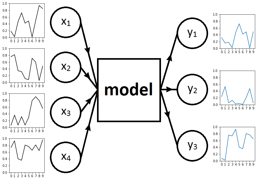
Fig. 1. Framework with input time series on the left, RNN model in the middle, and output time series on the right
Companion source code for this post is available here.
Description of the problem
We focus on the following problem. Let \(x_1, x_2, x_3, x_4\) four time series following the uniform distribution on \([0, 1]\). Each time series is indexed by \(\lbrace 0, 1, \ldots, T-1 \rbrace\).
Let \(y_1, y_2, y_3\) three time series defined as:
- \(y_1(t) = x_1(t-2)\) for \(t \geq 2\),
- \(y_2(t) = x_2(t-1) \times x_3(t-2)\) for \(t \geq 2\),
- \(y_3(t) = x_4(t-3)\) for \(t \geq 3\).
Each time series is also indexed by \(\lbrace 0, 1, \ldots, T-1 \rbrace\) (first undefined elements of \(y_1, y_2, y_3\) are sampled randomly).
Our task is to predict the three time series \(y = (y_1, y_2, y_3)\) based on inputs \(x = (x_1, x_2, x_3, x_4)\). To this end, we will train different RNN models. Fig. 1 represents the framework when \(T=10\).
Training and test sets
Two parameters are used to define training and test sets: \(N\) the number of sample elements and \(T\) the length of each time series. Each sample element consists of inputs \(x = (x_1, x_2, x_3, x_4)\) (four time series of length \(T\)) and outputs \(y = (y_1, y_2, y_3)\) (three time series of length \(T\)).
We take the same number of elements \(N\) in the training and the test set.
On the whole, for \(n \in \lbrace 0, ..., N-1 \rbrace\), the \(n\)-th element of the training set is: \((x^{n,\text{train}}, y^{n,\text{train}}),\) and the \(n\)-th element of the test set is: \((x^{n,\text{test}}, y^{n,\text{test}}).\)
For example, \(x^{n,\text{train}}_2(t) \in [0, 1]\) is the value at date \(t\) of the time series \(x^{n,\text{train}}_2\), which is the second input of \((x^{n,\text{train}}, y^{n,\text{train}})\), which is the \(n\)-th element of the training set.
This is implemented in function sample_time_series_roll.
Part A: Short time series with stateless LSTM
We consider short time series of length \(T = 37\) and sample size \(N = 663\).
In this part, the most difficult task is to reshape inputs and outputs correctly using numpy tools. We obtain inputs with shape \((N, T, 4)\) and outputs with shape \((N, T, 3)\).
Then, an classic LSTM model is defined and trained with \(10\) units.
##
# Model
##
model=Sequential()
dim_in = 4
dim_out = 3
nb_units = 10
model.add(LSTM(input_shape=(None, dim_in),
               return_sequences=True,
               units=nb_units))
model.add(TimeDistributed(Dense(activation='linear',
                                units=dim_out)))
model.compile(loss = 'mse', optimizer = 'rmsprop')

##
# Training
##
# 2 seconds for each epoch
np.random.seed(1337)
history = model.fit(inputs, outputs,
                    epochs = 500, batch_size = 32,
                    validation_data=(inputs_test,
                                     outputs_test))
plotting(history)
Training performs well (see Fig. 2), and after \(500\) epochs, training and test losses have reached \(0.0061\).
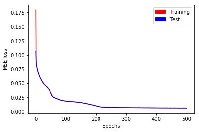
Fig. 2. MSE loss as a function of epochs for short time series with stateless LSTM
Results are also checked visually, here for sample \(n=0\) (blue for true output; orange for predicted outputs):
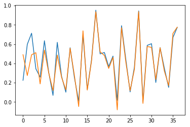
Fig. 3.a. Prediction of \(y_1\) for short time series with stateless LSTM
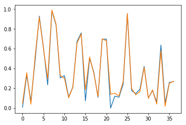
Fig. 3.b. Prediction of \(y_2\) for short time series with stateless LSTM
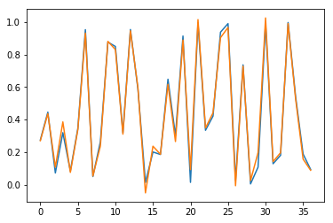
Fig. 3.c. Prediction of \(y_3\) for short time series with stateless LSTM
Conclusion of this part: Our LSTM model works well to learn short sequences.
Part B: Problem to predict long time series with stateless LSTM
We consider long time series of length \(T = 1443\) and sample size \(N = 17\). Note that product \(N \times T\) is the same in parts A and B (so computation of \(500\) epochs takes a similar amount of time).
We repeat the methodology described in part A in a simplified setting: We only predict \(y_1\) (the first time series output) as a function of \(x_1\) (the first time series input). Even in this case, predictions are not satisfactory after \(500\) epochs. Training and test losses have decreased to \(0.036\) (see Fig. 4), but it is not enough to give accurate predictions (see Fig. 5).
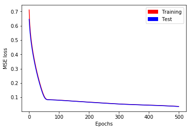
Fig. 4. MSE loss as a function of epochs for long time series with stateless LSTM
In Fig. 5, we check output time series for sample \(n=0\) and for the \(50\) first elements (blue for true output; orange for predicted outputs).
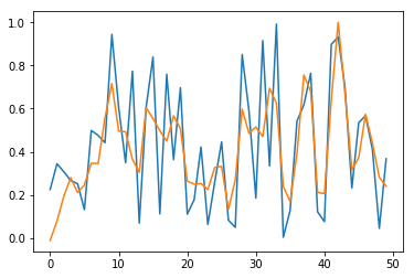
Fig. 5. Prediction for \(y_1\) for long time series with stateless LSTM, restricted to the \(50\) first dates
Conclusion of this part: Stateless LSTM models work poorly in practice for learning long time series, even for \(y_t = x_{t-2}\). The network is able to learn such dependence, but convergence is too slow. In this case, we need to switch to stateful LSTM as seen in part C.
Part C: Wrapper function to use stateful LSTM with time series
We have seen in part B that learning with LSTM can be very slow for long time series.
A natural idea is to cut the series into smaller pieces and to treat each one separately.
An issue arises by applying this method directly: Between two pieces, the network will reset hidden states, preventing share of information. For example, with \(y_1(t) = x_1(t-2)\) and a series cuts into \(2\) pieces, the first element of piece \(2\) cannot access to any information kept in memory from piece \(1\), and will be unable to produce a correct output.
Stateful LSTM
Here is coming stateful LSTM. We cut the series into smaller pieces, and also keep state of hidden cells from one piece to the next. This is illustrated in Fig. 6 with a series \(n=0\) of length \(T = 14\) divided into \(2\) pieces of length \(T_{\text{after_cut}} = 7\).

Fig. 6. a. Series before cut. Simplified workflow: Compute gradient of the series; Update parameters; Reset hidden states

Fig. 6. b. Series cut into \(2\) pieces of length \(7\). Simplified workflow with stateful LSTM: Compute gradient for piece \(1\); Update parameters; Keep hidden states; Compute gradient for piece \(2\); Update parameters; Reset hidden states
Considering batch size
In practice, we also need to pay attention of the batch size during cut.
The easiest case is when batch size is \(N\) the number of elements in the sample. In that case, we only reset states after each epoch.
Another simple case is when batch size is \(1\). In that case, we present each series in a lineup, and reset states after each series. This case is illustrated in Fig. 7.

Fig. 7. a. Series before cut. There are \(N = 3\) series of length \(T = 14\)

Fig. 7. b. Series after cut with \(\text{batch_size} = 1\) and \(T_{\text{after_cut}} = 7\)
The tricky case is when \(\text{batch_size} | N\) and \(\text{batch_size} \not \in \lbrace 1, N \rbrace\).
In that case, we present a cut batch series in a lineup, and reset states after a complete batch series.
This is illustrated in Fig. 8.
In the companion source code,
cut is done with stateful_cut function,
designed to manage number of cuts, batch size, as well as multiple inputs and outputs.

Fig. 8. a. Series before cut. There are \(N = 15\) series of length \(T = 14\)

Fig. 8. b. Series after cut. We have selected \(\text{batch_size} = 3\) and \(T_{\text{after_cut}} = 7\)
Part D: Long time series with stateful LSTM
We consider long time series of length \(T = 1443\) and sample size \(N = 16\).
We select \(\text{batch_size} = 8\) and \(T_{\text{after_cut}} = 37\). Consequently, we have: \(\text{nb_cuts} = T / T_{\text{after_cut}} = 39\).
After cut, we obtain inputs with shape \((N \times \text{nb_cuts}, T / \text{nb_cuts}, 4)\) i.e. \((624, 37, 3)\), and outputs with shape \((624, 37, 4)\).
Model
A stateful LSTM model in defined with \(10\) units.
##
# Model
##
nb_units = 10

model = Sequential()
model.add(LSTM(batch_input_shape=(batch_size, None, dim_in),
               return_sequences=True,
               units=nb_units,
               stateful=True))
model.add(TimeDistributed(Dense(activation='linear',
                                units=dim_out)))
model.compile(loss = 'mse', optimizer = 'rmsprop')
Training
For the training part,
a callback has been written to reset states after \(\text{nb_cuts}\) pieces
(function define_reset_states_class).
However, this callback is not properly called with validation data,
as noted by Philippe Remy on his blog.
Another function define_stateful_val_loss_class has been defined for that purpose.
Also, we need to take shuffle = False during model fitting.
On the whole, training is performed during \(100\) epochs as written in the following sample code. Training and test losses have decreased to \(0.002\) (see Fig. 9).
##
# Training
##
epochs = 100

nb_reset = int(N / batch_size)
nb_cuts = int(T / T_after_cut)
if nb_reset > 1:
    ResetStatesCallback = define_reset_states_class(nb_cuts)
    ValidationCallback = define_stateful_val_loss_class(inputs_test,
                                                        outputs_test,
                                                        batch_size, nb_cuts)
    validation = ValidationCallback()
    history = model.fit(inputs, outputs,
                        epochs = epochs, batch_size = batch_size,
                        shuffle=False,
                        callbacks = [ResetStatesCallback(), validation])
    history.history['val_loss'] = ValidationCallback.get_val_loss(validation)
else:
    # When nb_reset = 1, we do not need to reinitialize state
    history = model.fit(inputs, outputs,
                        epochs = epochs, batch_size = batch_size,
                        shuffle=False,
                        validation_data=(inputs_test,
                                         outputs_test))
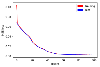
Fig. 9. MSE loss as a function of epochs for long time series with stateful LSTM
Predictions
Prediction with stateful model through Keras function model.predict needs a complete batch,
which is not convenient here.
Instead, we write a mime model: We take the same weights, but packed as a stateless model.
## Mime model which is stateless but contains stateful weights
model_stateless = Sequential()
model_stateless.add(LSTM(input_shape=(None, dim_in),
                         return_sequences=True, units=nb_units))
model_stateless.add(TimeDistributed(Dense(activation='linear',
                                          units=dim_out)))
model_stateless.compile(loss = 'mse', optimizer = 'rmsprop')
model_stateless.set_weights(model.get_weights())
Now, predictions are straighforward. Results are checked in Fig. 10 for sample \(n=0\) and for the \(100\) first elements (blue for true output; orange for predicted outputs):
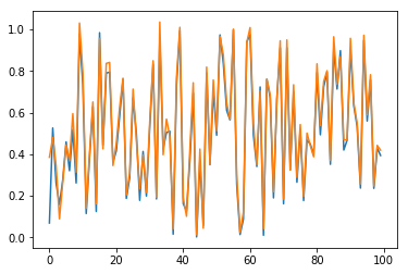
Fig. 10.a. Prediction of \(y_1\) for long time series with stateful LSTM, restricted to the \(100\) first dates
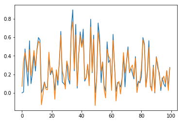
Fig. 10.b. Prediction of \(y_2\) for long time series with stateful LSTM, restricted to the \(100\) first dates
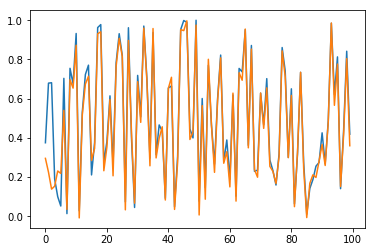
Fig. 10.c. Prediction of \(y_3\) for long time series with stateful LSTM, restricted to the \(100\) first dates
Conclusion of this part: Our stateful LSTM model works quite well to learn long sequences.
References
- Companion source code for this post
- Tutorial inspired from a StackOverflow question called “Keras RNN with LSTM cells for predicting multiple output time series based on multiple input time series”
- This post helps me to understand stateful LSTM
- To deal with part C in companion code, we consider a 0/1 time series as described by Philippe Remy in his post.