Periodic mixtures

Let \(f\) be a real function. For \(\lambda > 0\), we are interested in the equally-spaced summation \(\sum_{k=-\infty}^{+\infty} f(.+k\lambda)\), that can be interpreted depending on the context as a periodic mixture or as a wrapped distribution. For some specific functions such as the Gaussian density, we derive expressions, evaluations, and approximations of the sum, further accompanied with visualization of the different shapes for various values of \(\lambda\).

Read More

Divisibility of the exponential distribution

Let \(Z\) be a \(\text{Exp}(1)\) random variable. For \(\alpha_1, \ldots \alpha_N \in \mathbb{R}_{+}^{*}\), we are looking for variables \(X_1, \ldots X_N\) independent and following the same distribution such that:

\[Z = \sum_{j=1}^{N} \alpha_j X_j.\]

For the special case where all \(\alpha_j\) are equal, this corresponds to the problem of infinite divisibility of the exponential distribution, and in this case \(X_1\) follows \(\text{Gamma}(1/N, 1/\alpha_1)\), a gamma variable with shape \(1/N\) and scale \(1/\alpha_1\) (in particular when \(N=1\), we have \(X_1 \sim \text{Exp}(\alpha_1) = \text{Gamma}(1, 1/\alpha_1)\)).

We are willing to extend this divisibility property by deriving the characteristic function of \(X_1\) before inversing it numerically to retrieve the density. Some visualizations are provided.

Read More

RNN with Keras: Understanding computations

This tutorial highlights structure of common RNN algorithms by following and understanding computations carried out by each model. It is intended for anyone knowing the general deep learning workflow, but without prior understanding of RNN. If you really never heard about RNN, you can read this post of Christopher Olah first.

The present post focuses on understanding computations in each model step by step, without paying attention to train something useful. It is illustrated with Keras codes and divided into five parts:

  • TimeDistributed component,
  • Simple RNN,
  • Simple RNN with two hidden layers,
  • LSTM,
  • GRU.
Read More

RNN with Keras: Predicting time series

[This tutorial has been written for answering a stackoverflow post, and has been used later in a real-world context].

This tutorial provides a complete introduction of time series prediction with RNN.

In part A, we predict short time series using stateless LSTM. Computations give good results for this kind of series.

In part B, we try to predict long time series using stateless LSTM. In that case, model leads to poor results.

In part C, we circumvent this issue by training stateful LSTM. Stateful models are tricky with Keras, because you need to be careful on how to cut time series, select batch size, and reset states. I wrote a wrapper function working in all cases for that purpose.

In part D, stateful LSTM is used to predict multiple outputs from multiple inputs.

framework with T=10
Read More

Coal: Composition of Linear Functions

Coal is a small software dedicated to automatize composition of linear functions. For example, it can compute slope, intercept and fixed point of gfg given f: x ↦ ax+b and g: x ↦ cx+d. Here, a and b can be formal letters, rational values or real values.

example of data frame obtained with the code
Read More

Triangle pursuit

Let \(x_1, x_2, x_3\) be three points in a plane. We define \(x_4\) the point on the ray \([x_3 x_1)\) located at a distance \(1\) of \(x_3\). It is as \(x_1\) has been attracted to \(x_3\) but kept at distance. We continue by defining \(x_5\) the point on the ray \([x_4 x_2)\) located at a distance \(1\) of \(x_4\).

On the whole, we define from \((x_1, x_2, x_3)\) a recurrent sequence taking values in \(\mathbb{R}^2\) and such that, for \(n \geq 4\) (with \(N: x \mapsto \frac{x}{\| x \|}\) where \(\|.\|\) is a norm):

\[x_{n} = x_{n-1} - N(x_{n-1} - x_{n-3}).\]

We would like to study how behaves this sequence for large \(n\).

Rotation and one-norm Rotation and Euclidian norm Rotation and maximum norm
Read More

Computation of the gradient for SNE

Many methods exist to visualize high-dimensional data through a two-dimensional map. Those include linear techniques such as PCA and MDS; as well as nonlinear ones such as Isomap, LLE, SNE and t-SNE (resp. Principal Component Analysis, 1933; MultiDimensional Scaling, 1952; Isomap, 2000; Locally Linear Embedding, 2000; Stochastic Neighbor Embedding, 2002; t-Distributed Stochastic Neighbor Embedding, 2008). Some of those dimensionality reduction methods are illustrated in this sklearn example.

A popular method for nonlinear mapping is t-SNE. This method has been developed by Laurens van der Maaten and Geoffrey Hinton in [1]. It is based on SNE and improves it by addressing the “crowding problem” (tendency of mapped points to aggregate into a unique central cluster). You can familiarize yourself with t-SNE here, which allows exploration of various examples interactively.

In this post, we propose to derive gradient of the SNE algorithm (not to be confused with t-SNE, for which gradient calculation is detailed in Appendix A of [1]). SNE gradient is given in both original and t-SNE article, but neither detailed (see Equation 5 of [2], and Section 2 of [1]).

Intro illustration with cost and its gradient for SNE
Read More

Maximizing likelihood is equivalent to minimizing KL-divergence

This post explains why maximizing likelihood is equivalent to minimizing KL-divergence. This can already be found here and here, but I restate this in my “own” words.

More generally, I encourage you to read Section 3.13 of Deep Learning book for insights on information theory.

Let \(\mathbf{x} = (x_1, \ldots x_n)\) a dataset of \(n\) elements.

We assume that each \(x_i\) has been sampled independently from a random variable \(X\) with density \(p = p_{\theta_0}\) and corresponding to a true (unknown and fixed) parameter \(\theta_0\).

We let \(q = p_{\theta}\) the density function corresponding to another parameter \(\theta\).

The likelihood of \(\mathbf{x}\) given \(\theta\) is \(L_{\theta}(\mathbf{x}) = \prod_{i = 1}^n p_{\theta}(x_i)\).

The opposite of log-likelihood divided by \(n\) is:

\[-\frac{1}{n} \log L_{\theta}(\mathbf{x}) = -\frac{1}{n} \sum_{i=1}^n \log p_{\theta}(x_i) \xrightarrow[n \rightarrow +\infty]{} E_{\theta_0} \left[ - \log p_{\theta}(X) \right],\]

and

\[E_{\theta_0} \left[ - \log p_{\theta}(X) \right] = - \int \log p_{\theta}(x) dp_{\theta_0}(x) = - \int \log q(x) dp(x) =: H(p, q).\]

In the previous equation, \(H(p, q)\) stands for the (continuous) cross-entropy between \(p\) and \(q\). We let \(H(p)\) the (continuous) entropy of \(p\) and \(\text{KL}(p \mid \mid q)\) the Kullback-Leibler divergence between \(p\) and \(q\).

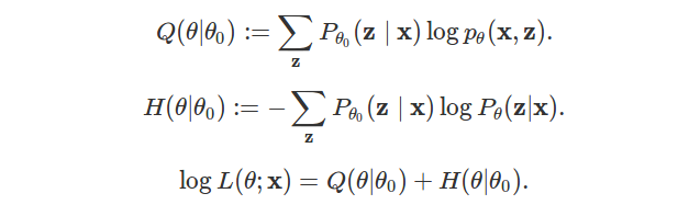
Since \(H(p, q) = H(p) + \text{KL}(p \mid \mid q)\), maximizing likelihood is equivalent to minimizing KL-divergence.

Read More

Optimizing GMM parameters using EM

A Gaussian Mixture Model (GMM) models data as a finite mixture of Gaussians. It is often used to perform clustering. In this case, the number of Gaussians \(K\) is the number of clusters and is initially selected. Compared to \(K\)-means, GMM allows clusters with uneven variance and density.

Parameters are usually estimated using an Expectation-Maximization (EM) algorithm, its aim being to iteratively increase likelihood of the dataset. GMM is actually a perfect model to understand how EM is working.

2D dataset to cluster 2D dataset after GMM clustering
Read More

Rediscover EM algorithm from scratch

Expectation-Maximization algorithm (EM) is an algorithm used to estimate parameters of statistical models comprising latent variables. It is applied in the case where direct calculation of maximum likelihood estimation (MLE) is impractical. EM updates parameters of the model iteratively, in order to increase likelihood of the set. It generally gives good estimation results, although there is no guarantee of convergence to MLE.

Many introductions of EM exist on the web. This one starts from the likelihood computation problem and uses inductive reasoning to bring out EM. No implementation is provided.

We begin by describing a general model involving latent variables. We then explain why direct computation of MLE is intractable. After that, ideas are introduced one by one and lead us naturally towards EM. Those ideas are formalized afterwards, making EM a practical algorithm to estimate parameters.

Intro illustration with decomposition of log-likelihood in EM
Read More

Langton's ant extended to Voronoi tessellations

Langton’s ant is a cellular automaton driven by a simple set of rules and running on a square lattice. It is one of the most simple system leading to an emergent behavior. In this post, the system is extended to run on any Voronoi tessellation of the plane. Simulations show interesting walks for some partitions of the plane, including chaotic structures, highway patterns and even bounded evolutions.

Bounded evolution of the ant
Read More

An illustration of Metropolis–Hastings algorithm

Metropolis–Hastings algorithm is a method for sampling from a probability distribution. It is used when direct sampling is difficult.

This post illustrates the algorithm by sampling from \(\mathcal{N}(. \mid > 5)\) – the univariate normal distribution conditional on being greater than \(5\). This example has been chosen for its simplicity, for understanding how the algorithm actually works.

For real applications, other methods are preferred for sampling \(\mathcal{N}(. \mid > l)\): It is direct for \(l = 5\), and more tricky when \(l\) is larger than \(10\). You can read this Wikipedia section for details.

Simulation code has been written in R and is available at that address.

Resulting sample of normal distribution conditional on being greater than 5
Read More

Clickstream

In this post, we explore data collected with Anabasis webapp. 144674 records have been retrieved consisting of date, picture number, cell position and user id. We derive density plots from data to deduce where players prefer to click. Afterwards, we show how players share the work together on some selected pictures.

density inside room (top 5000 for each draw)
Read More

Anabasis webapp

Anabasis is a webapp where players can draw collaborative paintings. Each draw stands on a board containing ten thousand cells. Every player contributes at the same time on the same drawing. When a player clicks on a dark cell, it transforms to a light cell.

The work is finished when one special cell among ten thousand has been found. At this moment, the lucky player can choose the name of the draw. Finished artworks are therefore available in the draws section.

title screen of the game

Click on the screen to launch the game in your browser. The loading may take some seconds.

I released this webapp as a challenge to understand how node.js and mongodb are working. I deployed the app with Heroku and MongoLab. The whole source is available in my github! Analysis of data collected with the app is available here.

Read More

Bank vault holdup webapp

Bank vault holdup is a game where you have to guess a secret pass to open the bank vault and get the reward! There is no hint, you just have to follow your intuition.

title screen of the game

Click on the screen to launch the game in your browser. The loading may take some seconds.

Read More

Nim function for take-a-prime game

The Nim function for take-a-prime game is a math sequence with interesting patterns. We define this sequence \((u_n)\) recursively. For all \(n\) in \(\mathbb{N}\) (the set of non-negative integers), \(u_n\) is the lowest number in \(\mathbb{N}\) such that for all prime numbers \(p\) (with \(n-p \geq 0\)), \(u_n \neq u_{n-p}\).

first elements of the sequence
Read More

Trigger snake

Trigger snake is a snake game with new features, making it fast, lively and challenging. You can download it here (Windows), or compile C++/Qt4 sources yourself. The software contains a component to display graphical statistics in-game. It can be used to follow player’s behavior, for example by showing preference to some regions or directions.

introduction picture of the game
Read More

Packing cubes

How to make a 3×3×3 cube with six 2×2×1 cuboids and three 1×1×1 cubes, i.e. to show the following “equation”? You can move them, change their orientation, but splitting is not allowed.

packingCubesImage

Read More

Gender of French nouns

Like other Romance languages, French nouns are divided in two almost distinct genders: feminine and masculine. Deciding the gender of a word is not obvious. For example, a table is feminine (“une table”) but an acid is masculine (“un acide”).

On the following plots, we check out the distribution of the gender across the letters. We then learn a simple tip to choose the gender of an unknown noun.

genderLetterIntro

Read More

Description and modeling of FlapMMO score data

FlapMMO is an online game similar to Flappy Bird. The player controls a bird and the aim is to fly as far as possible, avoiding the pipes. At the same time, you see other players playing.

flappy1

In this post, an exploration of a dataset of scores is performed, using descriptive statistics and testing some probabilistic models.

Read More

Tutorial for using a computer cluster

Using a computer cluster to run some program is useful if your program needs:

  • a large amount of CPU or memory resources,
  • to run during a large amount of time.

In those cases, you can follow this short tutorial, designed for the ICJ cluster.

apercuClusters4
Read More

Watering and draining planets

What the Earth would look like if the sea level suddenly changed? And what would be the Moon, Mars and Venus with as much water as on the Earth? Show this on the following maps and compare our Earth with other astronomical objects.

World maps. On this first map, we can show how the world would be if the sea level increased by +100m. 100m increase of the sea level

Read More